Let’s Think in Graphs: Introduction to Graph Theory and its Applications using Python
Introduction
“There is a magic in graphs. The profile of a curve reveals in a flash a whole situation — the life history of an era of prosperity. The curve informs the mind, awakens the imagination, convinces.”
– Henry D. Hubbard
Visualizations are a powerful way to simplify and interpret the underlying patterns in data. The first thing I do, whenever I work on a new dataset is to explore it through visualization. And this approach has worked well for me. Sadly, I don’t see many people using visualizations as much. That is why I thought I will share some of my “secret sauce” with the world!
Use of graphs is one such visualization technique. It is incredibly useful and helps businesses make better data-driven decisions. But to understand the concepts of graphs in detail, we must first understand it’s base – Graph Theory.
In this article, we will be learning the concepts of graphs and graph theory. We will also look at the fundamentals and basic properties of graphs, along with different types of graphs.
We will then work on a case study to solve a commonly seen problem in the aviation industry by applying the concepts of Graph Theory using Python.
Let’s get started!
Table of Contents
- Introduction to Graphs
- Why Graphs?
- Origin of Graph theory: Seven Bridges of Königsberg
- Fundamentals of Graphs
- Basic Properties and Terminologies Related to Graphs
- Types of Graphs
- Continuing the Problem of the Seven Bridges of Königsberg
- Introduction to Trees
- Graph Traversal
- Implementing Graph Theory Concepts to Solve an Airlines Challenge
Introduction to Graphs
Consider the plot shown below:
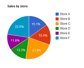
It’s a nice visualization of the store-wise sales of a particular item. But this isn’t a graph, it’s a chart. Now you might be wondering why is this a chart and not a graph, right?
Well, a chart represents the graph of a function. Let me explain this by expanding on the above example.
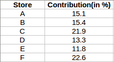
Out of the total units of a particular item, 15.1% are sold from store A, 15.4% from store B, and so on. We can represent it using a table:
Corresponding to each store is their contribution (in %) to the overall sales. In the above chart, we mapped store A with 15.1% contribution, store B with 15.4%, so on and so forth. Finally, we visualized it using a pie chart. But then what’s the difference between this chart and a graph?
To answer this, consider the visual shown below:
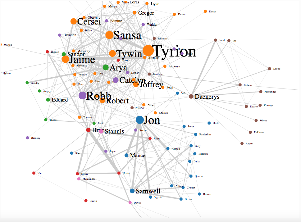
The points in the above visual represent the characters of Game of Thrones, while the lines joining these points represent the connection between them. Jon Snow has connections with multiple characters, and the same goes for Tyrion, Cersei, Jamie, etc.
And this is what a graph looks like. A single point might have connections with multiple points, or even a single point. Typically, a graph is a combination of vertices (nodes) and edges. In the above GOT visual, all the characters are vertices and the connections between them are edges.
We now have an idea of what graphs are, but why do we need graphs in the first place? We’ll look at this pertinent question in the next section.
Why Graphs?
Suppose you booked an Uber cab. One of the most important things that is critical to Uber’s functioning is its ability to match drivers with riders in an efficient way. Consider there are 6 possible rides that you can be matched with. So, how does Uber allocate a ride to you? We can make use of graphs to visualize how the process of allotting a ride might be:
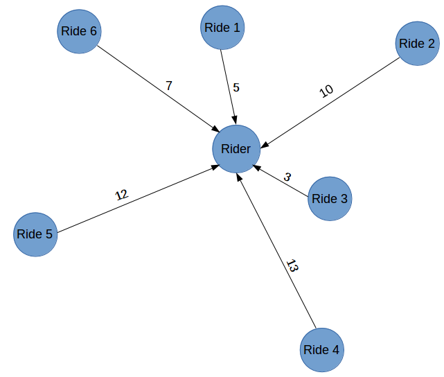
As you can interpret, there are 6 possible rides (Ride 1, Ride 2, …. Ride 6) which the rider can be matched with. Representing this in graph form makes it easier to visualize and finally fulfill our aim, i.e., to match the closest ride to the user. The numbers in the above graph represent the distance (in kilometers) between the rider and his/her corresponding ride. We (and of course Uber) can clearly visualize that Ride 3 is the closest option.
Note: For simplicity, I have taken only the distance metric to decide which ride will be allotted to the rider. Whearas in a real life scenario, there are multiple metrics through which the allotment of a ride is decided, such as rating of the rider and driver, traffic between different routes, time for which the rider is idle, etc.
Similarly, online food delivery aggregators like Zomato can select a rider who will pick up our orders from the corresponding restaurant and deliver it to us. This is one of the many use cases of graphs through which we can solve a lot of challenges. Graphs make visualizations easier and more interpretable.
To understand the concept of graphs in detail, we must first understand graph theory.
Origin of Graph theory: Seven Bridges of Königsberg
We’ll first discuss the origins of graph theory to get an intuitive understanding of graphs. There is an interesting story behind its origin, and I aim to make it even more intriguing using plots and visualizations.
It all started with the Seven Bridges of Königsberg. The challenge (or just a brain teaser) with Königsberg’s bridges, was to be able to walk through the city by crossing all the seven bridges only once. Let us visualize it first to have a clear understanding of the problem:
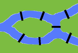
Give it a try and see if you can walk through the city with this restraint. You have to keep two things in mind while trying to solve the above problem (or should i say riddle?):
- You cannot uncross any bridge
- Each bridge must not be crossed more than once
You can try any number of combinations, but it remains an impossible challenge to crack. There is no way in which one can walk through the city by crossing each bridge only once. Leonhard Euler delved deep into this puzzle to come up with the reason why this is such an impossible task. Let’s analyze how he did this:
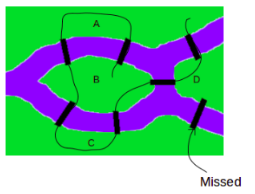
There are four distinct places in the above image: two islands (B and D), and two parts of the mainland (A and C) and a total of seven bridges. Let us first look at each land separately and try to find patterns (if any exist at all) :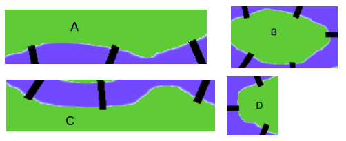
One inference from the above image is that each land is connected with an odd number of bridges. If you wish to cross each bridge only once, then you can enter and leave a land only if it is connected to an even number of bridges. In other words, we can generalize that if there are even number of bridges, it’s possible to leave the land, while it’s impossible to do so with an odd number.
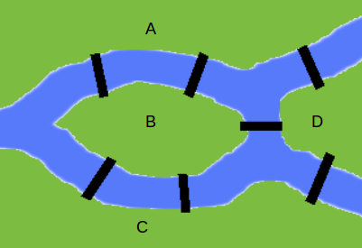
Let’s try to add one more bridge to the current problem and see whether it can crack open this problem: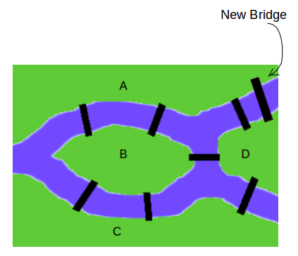
Now we have 2 lands connected with an even number of bridges, and 2 lands connected with an odd number of bridges. Let’s draw a new route after the addition of the new bridge: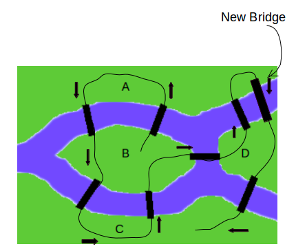
The addition of a single bridge solved the problem! You might be wondering if the number of bridges played a significant part in solving this problem? Should it be even all the time? Well, that’s not always the case. Euler explained that along with the number of bridges, the number of pieces of land with an odd number of connected bridges matters as well. Euler converted this problem from land and bridges to graphs, where he represented the land as vertices and the bridges as edges: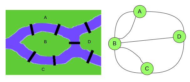
Here, the visualization is simple and crystal clear. Before we move further and delve deeper into this problem, let us first understand the fundamentals and basic properties of a graph.
Fundamentals of Graphs
There are many key points and key words that we should keep in mind when we are dealing with graphs. In this section, we will discuss all those keywords in detail.
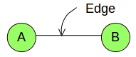
- Vertex: It is a point where multiple lines meet. It’s also known as the node.
 A vertex is generally denoted by an alphabet as shown above.
 - Edge: It is a line that connects two vertices.
- Graph: As discussed in the previous section, graph is a combination of vertices (nodes) and edges. G = (V, E) where V represents the set of all vertices and E represents the set of all edges of the graph.

- Degree of Vertex: The degree of a vertex is the number of edges connected to it. In the below example, Degree of vertex A, deg(A) = 3Degree of vertex B, deg(B) = 2.
- Parallel Edge: If two vertices are connected by more than one edge, then these edges are called parallel edges.

- Multi Graph: These are the graphs which have parallel edges:
These are some of the fundamentals which you must keep in mind when dealing with graphs. Now onto understanding the basic properties of a graph.
Basic properties and terminologies related to Graphs
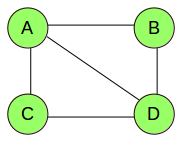
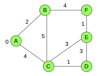
So far, we have seen what a graph looks like and it’s different components. Now we will turn our focus to some basic properties and terminologies related to a graph. We will be using the below given graph (referred to as G) and understand each terminology using the same:
Take a moment and think about possible solutions to the following questions:
- How far is a vertex from the other vertices of a graph?
- What is the maximum distance between a vertex and all the other vertices?
- Is there any vertex which is closest to all the other vertices? If so, what is that shortest distance?
- What is the central point of the graph?
I will try to answer all these questions using basic graph terminologies:
- Distance between two Vertices : It is the number of edges in the shortest path between two vertices. Let us try to calculate the distance between vertices A and D:
Possible paths between A and D are:
AB -> BC -> CD
AD
AB -> BD
Out of these three paths, AD is the shortest having only one edge. Hence, the distance between A and D is 1.
Similarly, we can calculate the distance between each pair of vertices. So, this answered our first question of determining the distance between any pair of vertices.
- Eccentricity of a Vertex : It is the maximum of distances between a vertex to all other vertices. To calculate eccentricity of any vertex, we must know the distance between that vertex to all other vertices. Let’s calculate the eccentricity for vertex A. So, the distances are:
Distance between A and B – 1
Distance between A and C – 2
Distance between A and D – 1
Maximum of all these distances is the eccentricity of a vertex.
Eccentricity of A, e(A) = 2
When the eccentricity of a vertex is high, it means that there are vertices that are far away from that vertex. This answers our second question where we aimed to calculate the maximum of distances between a vertex to all the other vertices.
- Radius of a connected Graph : Minimum eccentricity of all the vertices of a graph is referred as the Radius of that graph. We first have to calculate the eccentricity for each vertex. Try to calculate the eccentricity on your own and if you find any difficulty in calculations, feel free to ask in the comment section.The eccentricity for all the vertices is:
e(A) = 2
e(B) = 1
e(C) = 2
e(D) = 1
Minimum value of the eccentricity for all the vertices is the radius of that graph. In our case minimum eccentricity is 1 and hence the radius of the graph is:
r(G) = 1
It tells us the distance of a vertex which is the closest to all other vertices.
- Diameter of a connected Graph : Radius of a graph is the minimum value of the eccentricity for all the vertices, similarly, Diameter of a graph is the maximum value of the eccentricity for all the vertices. In our case the Diameter of the graph is:
d(G) = 2
- Central point of a graph : Vertex for which the eccentricity is equal to the radius of the graph is known as central point of the graph. A graph can have more than one central point as well. In our case the Radius of the graph is 1 and the vertices with eccentricity equals to 1 are B and D. Hence ‘B’ and ‘D’ are the central points of graph G.
This answers our last question of determining the central point of a graph. Consider an example of airport connectivity graph. So, an airport which is connected to most number of other airports can be considered as the central airport.
These are some of the terminologies related to graphs. Next we will discuss the different types of graphs.
Types of Graphs
There are vairous and diverse types of graphs. In this section, we will discuss some of the most commonly used ones.
- Null Graph: These are the graphs which do not contain any edges.
There is no connection between the vertices.
- Non-Directed Graph: These are the graphs which have edges, but these edges do not have any particular direction.
- Directed Graph: When the edges of a graph have a specific direction, they are called directed graphs.
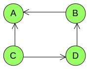
Consider the example of Facebook and Twitter connections. When you add someone to your friend list on Facebook, you will also be added to their friend list. This is a two-way relationship and that connection graph will be a non-directed one. Whereas if you follow a person on Twitter, that person might not follow you back. This is a directed graph.
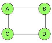
- Connected Graph: When there is no unreachable vertex, i.e., there exists a path between every pair of vertices, such graphs are called connected graphs.
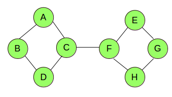
- Disconnected Graph: These are those graphs which have unreachable vertex(s), i.e., a path does not exist between every pair of vertices.
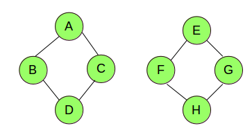 If a graph is connected, then there is always a path from each vertex to all the other vertices of that graph. While if a graph is disconnected, there will always be at least one vertex which will not have connections with all the other vertices of the graph. This can help the airlines to decide whether all the airports are connected or not. They can visualize the connections, and if there is any unconnected airport, new flights can be introduced to improve on the existing situation.
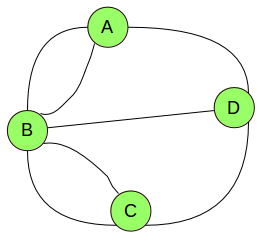
- Regular Graph: When all the vertices in a graph have the same degree, these graphs are called k-Regular graphs (where k is the degree of any vertex). Consider the two graphs shown below:
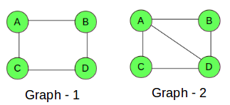
- For Graph – 1, the degree of each vertex is 2, hence Graph – 1 is a regular graph. Graph-2 is not a regular graph as the degree of each vertex is not the same (for A and D degree is 3, while for B and D it’s 2).
Now that we have an understanding of the different types of graphs, their components, and some of the basic graph-related terminologies, let’s get back to the problem which we were trying to solve, i.e. the Seven Bridges of Königsberg. We shall explore in even more detail how Leonhard Euler approached and explained his reasoning.
Continuing the problem of the Seven Bridges of Königsberg
We saw earlier that Euler transformed this problem using graphs:
Here, A, B, C, and D represent the land, and the lines joining them are the bridges. We can calculate the degree of each vertex.
deg(B) = 5
deg(A) = deg(C) = deg(D) = 3
Euler showed that the possibility of walking through a graph (city) using each edge (bridge) only once, strictly depends on the degree of vertices (land). And such a path, which contains each edge of a graph only once, is called Euler’s path.
Can you figure out Euler’s path for our problem? Let’s try!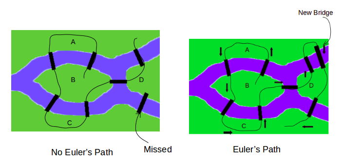
And this is how the classic Seven Bridges of Königsberg challenge can be solved using graphs and Euler’s path. And this is basically the origin of Graph Theory. Thanks to Leonhard Euler!
Introduction to Trees
Trees are one of the most powerful and effective ways of representing a graph. In this section, we will learn what binary search trees are, how they work, and how they make visualizations more interpretable. But before all that, take a moment to understand what trees actually are in this context.
Trees are graphs which do not contain even a single cycle:
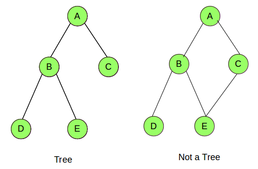
In the above example, the first graph has no cycle (aka a tree), while the second graph has a cycle (A-B-E-C-A, hence it’s not a tree).
The elements of a tree are called nodes. (A, B, C, D, and E) are the nodes in the above tree. The first node (or the topmost node) of a tree is known as the root node, while the last node (node C, D and E in the above example) is known as the leaf node. All the remaining nodes are known as child nodes (node B in our case).
It’s time to move on to one of the most important topics in Graph Theory, i.e., Graph Traversal.
Graph Traversal
Suppose we want to identify the location of a particular node in a graph. What might me the possible solution to identify nodes of a graph? How to start? What should be the starting point? Once we know the starting point, how to proceed further? I will try to answer all these questions in this section by explaining the concepts of Graph Traversal.
Graph Traversal refers to visiting every vertex and edge of a graph exactly once in a well-defined order. As the aim of traversing is to visit each vertex only once, we keep a track of vertices covered so that we do not cover same vertex twice. There are various methods for graph traversal and we will discuss some of the famous methods:
- Breadth First Search
We start from the source node (root node) and traverse the graph, layer wise. Steps for Breadth First Search are:
- First move horizontally and visit all the nodes of current layer.
- Move to the next layer and repeat the steps done above.
Let me explain it with a visualization:
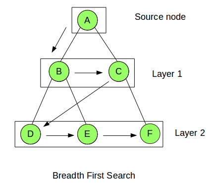
So in Breadth First Search, we start from the Source Node (A in our case) and move down to the first layer, i.e. Layer 1. We cover all the nodes in that layer by moving horizontally (B -> C). Then we go to the next layer, i.e. Layer 2 and repeat the same step (we move from D -> E -> F). We continue this step until all the layers and vertices are covered.
Key advantage of this approach is that we will always find the shortest path to the goal. This is appropriate for small graphs and trees but for more complex and larger graphs, its performance is very slow and it also takes a lot of memory. We will look at another traversing approach which takes less memory space as compared to BFS.
- Depth First Search
Let us first look at the steps involved in this approach:
- We first pick the source node and store all its adjacent nodes.
- We then pick up a node from stored nodes and store all its adjacent nodes.
- This process is repeated until no node is available.
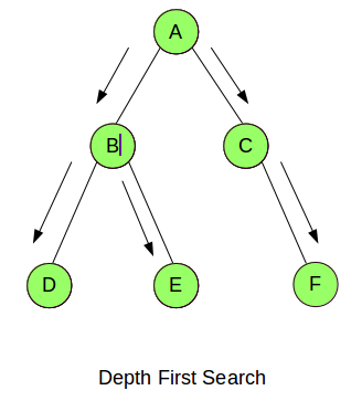
The sequence for Depth First Search for the above example will be:
A -> B -> D -> E -> C -> F
Once a path has been fully explored it can be removed from memory, so DFS only needs to store the root node, all the children of the root node and where it currently is. Hence, it overcomes the memory problem of BFS.
- Binary Search Tree
In this approach all the nodes of a tree are arranged in a sorted order. Let’s have a look at an example of Binary Search Tree:
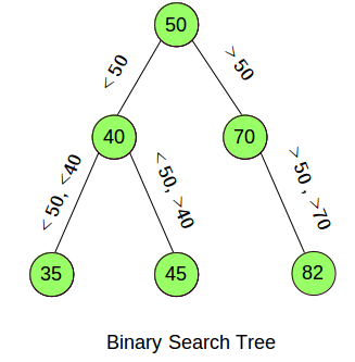
As mentioned earlier, all the nodes in the above tree are arranged based on a condition. Suppose we want to access the node with value 45. If we would have followed BFS or DFS, we would have required a lot of computational time to reach to it. Now let’s look at how a Binary Search Tree will help us to reach to the required node using least number of steps. Steps to reach to the node with value 45 using Binary Search Tree:
- We start with the root node, i.e. 50.
- Now 45 is less than 50 (45 < 50), so we move to the left of root node.
- We then compare the values. As it turns out 45 is greater than 40 (45 > 40), so we move to the right of that node.
- Here we are at the node with value 45.
This approach is very fast and takes very less memory as well. Most of the concepts of Graph Theory have been covered. Next, we will try to implement these concepts to solve a real-life problem using Python.
Implementing Graph Theory in Python to Solve an Airlines Challenge
And finally, we get to work with data in Python! In this dataset, we have records of over 7 million flights from the USA. The below variables have been provided:
- Origin and destination
- Scheduled time of arrival and departure
- Actual time of arrival and departure
- Date of the journey
- Distance between the source and destination
- Total airtime of the flight
It is a gigantic dataset and I have taken only a sample from it for this article. The idea is to give you an understanding of the concepts using this sample dataset, and you can then apply them to the entire dataset. Download the dataset which we will be using for the case study from here. We will first import the usual libraries, and read the dataset, which is provided in a .csv format:
import pandas as pd
import numpy as np
data = pd.read_csv('data.csv')
Let’s have a look at the first few rows of the dataset using the head() function:
data.head()
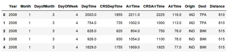
Here, CRSDepTime, CRSArrTime, DepTime, and ArrTime represent the scheduled time of departure, the scheduled time of arrival, the actual time of departure, and the actual time of arrival respectively. Origin and Dest are the Origin and Destination of the journey.
There can often be multiple paths from one airport to another, and the aim is to find the shortest possible path between all the airports. There are two ways in which we can define a path as the shortest:
- By distance
- By air time
We can solve such problems using the concepts of graph theory which we have learned so far. Can you recall what we need to do to make a graph?
The answer is identifying the vertices and edges! We can convert the problem to a graph by representing all the airports as vertices, and the route between them as edges. We will be using NetworkX for creating and visualizing graphs. NetworkX is a Python package for the creation, manipulation, and study of the structure, dynamics, and functions of complex networks. You can refer to the documentation of NetworkX here.
After installing NetworkX, we will create the edges and vertices for our graph using the dataset:
import networkx as nx
df = nx.from_pandas_edgelist(data, source='Origin', target='Dest', edge_attr=True)
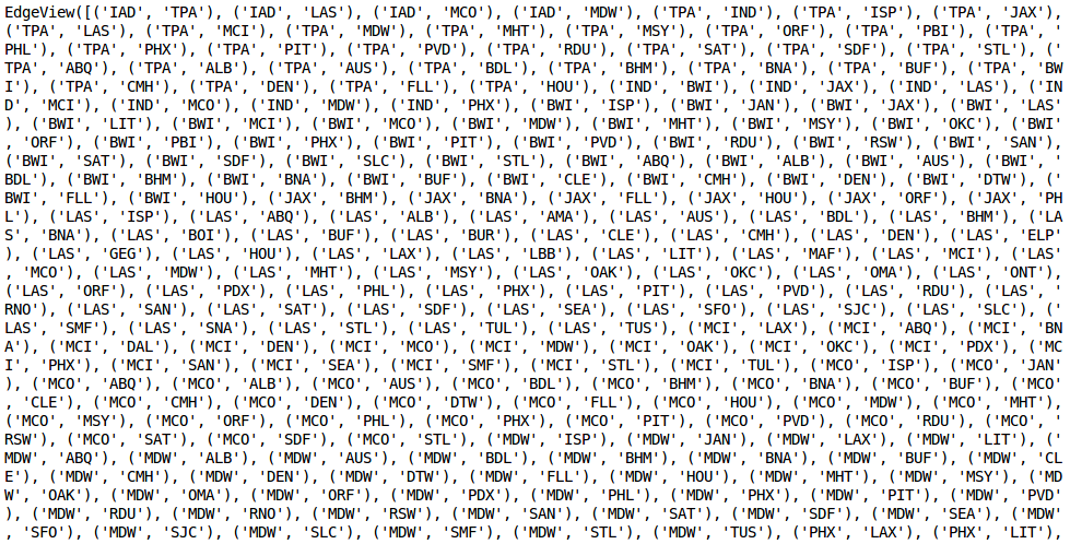
It will store the vertices and edges automatically. Take a quick look at the edges and vertices of the graph which we have created:
df.nodes()

df.edges()
Let us plot and visualize the graph using the matplotlib and draw_networkx() functions of networkx.
import matplotlib.pyplot as plt
% matplotlib inline

plt.figure(figsize=(12,8))
nx.draw_networkx(df, with_labels=True)
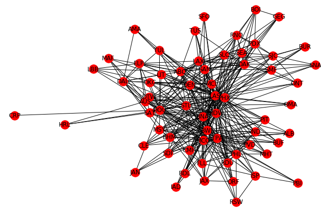
The above amazing visualization represents the different flight routes. Suppose a passenger wants to take the shortest route from AMA to PBI. Graph theory comes to the rescue once again!
Let’s try to calculate the shortest path based on the airtime between the airports AMA and PBI. We will be using Dijkstra’s shortest path algorithm. This algorithm finds the shortest path from a source vertex to all the vertices of the given graph. Let me give you a brief run through of the steps this algorithm follows:
- Creates a sptSet (Shortest Path Tree Set) which keeps track of vertices included in the shortest path tree, i.e., minimum distance from the source vertex is calculated and finalized. Initially, this set is empty.
- Assign a distance value to all vertices in the input graph. We assign a value of 0 to the source vertex and a value of INFINITE to all the remaining vertices.
- Until the sptSet does not include all the vertices, we follow these sub-steps:
- Pick a vertex which is not in the sptSet and is closest to the source vertex
- Include that vertex in the sptSet
- Update the distances of all adjacent vertices
Let us take an example to understand this algorithm in a better way:
Here the source vertex is A. The numbers represent the distance between the vertices. Initially, the sptSet is empty so we will assign distances to all the vertices. The distances are:
{0, INF, INF, INF, INF, INF}, where INF represents INFINITE.
Now, we will pick the vertex with the minimum distance, i.e., A and it will be included in the sptSet. So, the new sptSet is {A}. The next step is to pick a vertex which is not in the sptSet and is closest to the source vertex. This, in our case, is B with a distance value of 2. So this will be added to the sptSet.
sptSet = {A,B}
Now we will update the distances of vertices adjacent to vertex B:
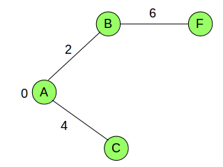
The distance value of the vertex F becomes 6. We will again pick the vertex with the minimum distance value which is not already included in SPT (C with a distance value of 4).
sptSet = {A,B,C}
We will follow similar steps until all the vertices are included in the sptSet. Let’s implement this algorithm and try to calculate the shortest distance between the airports. We will use the dijkstra_path() function of networkx to do so:
shortest_path_distance = nx.dijkstra_path(df, source='AMA', target='PBI', weight='Distance')
Shortest_path_distance
![]()
This is the shortest possible path between the two airports based on the distance between them. We can also calculate the shortest path based on the airtime just by changing the hyperparameter weight=’AirTime’:
shortest_path_airtime = nx.dijkstra_path(df, source='AMA', target='PBI', weight='AirTime')
shortest_path_airtime
![]()
This is the shortest path based on the airtime. Intuitive and easy to understand, this was all about graph theory!
End Notes
This is just one of the many applications of Graph Theory. We can apply it to almost any kind of problem and get solutions and visualizations. Some of the application of Graph Theory which I can think of are:
- Finding the best route for delivering posts
- Representing networks of communication. For example, link structure of a website can be represented using directed graphs.
- Determining the social behaviour of a person using their social connection graph
- Travel planning as discussed in the airlines case study
These are some of the applications. You can come up with many more. Feel free to share them in the comment section below. We also have multiple articles related to graphs and networks as listed below:
- Knowledge Graph for Information Mining
- Find Similar Web Pages using Graphs
- Link Prediction in Social Networks
- Network Analysis in Cricket
I hope you have enjoyed the article. Looking forward to your responses.
My research interests lies in the field of Machine Learning and Deep Learning. Possess an enthusiasm for learning new skills and technologies.


Awesome Article. Written in an intuitive and lucid manner.
Thank you Ankur!
Thanks Pulkit for the post. Did you find any way of drawing edge thickness?
Glad you liked the article! There is a concept called weighted graphs in which you can give weights to edges. For more details on this, refer here.
Pulkit, Well written! It is a good introduction to the computer science students. Python integration is excellent. However, I think the quote of Henry D. Hubbard is not on graphs of Graph Theory bu t is on the graph created out of a function.
Hi Joseph, Thanks for the feedback. I just added that quote to get an intuition of how graphs can be useful for visualization.
Great article! Will there be others? It would be great if you could point some books and courses about it too in the end of the article.
Hi, Glad you liked the article!! You can refer "Introduction to Graph Theory" course of coursera to learn more about graph theory.
Thanks for this nice article. I have some question as below. 1) Can we implemented travelling sales man problem using graph theory in python? 2) Need some more example of Real life project case study.
Hi Ashish, 1. To solve the traveling salesman problem, you can consider the cities as vertices and the distance between them as edges. Then you can solve it using Graph Theory. For more details, refer here. 2. For projects related to Graph Theory, you can refer these links: http://freshmeat.sourceforge.net/tags/graph-theory http://slogix.in/projects-in-social-networks
Hi Pulkit, you explained this in such a nice way, loved going through it. There is one small typo, I think, and you may correct. "...while the second graph has a cycle (A-B-E-C-E, hence it’s not a tree)" should be "... (A-B-E-C-A, hence it’s not a tree)". Thank you.
Hi Gautam, Thanks for pointing it out. I have changed the same.
Great Explanation of Graph Theory using such beautiful examples.A worthy article to bookmark.
Thank you Krishna!
Man, this is a great post! Perhaps add more sentences about how to do more visualization in the graph (or network) would be a huge PLUS!!! Anyway, this is super!!! Have become one of your fans now. ; )
Hi, Thanks for the feedback. Will work on that and update it in the article.
This is a grear post, only one question, is there a github link or a code snippet for the airlines problem so we could actually play around with it? Great article and great explaining :D
Excellent summary for anyone looking to understand basics of graph, keep adding more problems, use cases, etc especially on predicting rare cases using graph theory
Thank you Sunil!
Hello! Here I am reading and trying the implement the work in Python but the dataset hyperlink says there is no such thing there. Could you provide another link or tell me where to find this dataset please? Thank you.
Thanks for your great post!, I'm new in python, Could you please let me know the shortest path to learn community search over attributed and weighted graphs using python.
Thank you for this nice article. When I try to dowload the datset, It's no longer available. Please, can you sent it to me? Thank you very much.