Nuts & Bolts of Reinforcement Learning: Model Based Planning using Dynamic Programming

Introduction

Deep Reinforcement learning is responsible for the two biggest AI wins over human professionals – Alpha Go and OpenAI Five. Championed by Google and Elon Musk, interest in this field has gradually increased in recent years to the point where it’s a thriving area of research nowadays.

In this article, however, we will not talk about a typical RL setup but explore Dynamic Programming (DP). DP is a collection of algorithms that  can solve a problem where we have the perfect model of the environment (i.e. probability distributions of any change happening in the problem setup are known) and where an agent can only take discrete actions.

DP essentially solves a planning problem rather than a more general RL problem. The main difference, as mentioned, is that for an RL problem the environment can be very complex and its specifics are not known at all initially for machine learning.

But before we dive into all that, let’s understand why you should learn dynamic programming in the first place using an intuitive example.Also , these Programming will help you to understand q-learning.

Why learn dynamic programming?

Apart from being a good starting point for grasping reinforcement learning, dynamic programming can help find optimal solutions to planning problems faced in the industry, with an important assumption that the specifics of the environment are known. DP presents a good starting point to understand RL algorithms that can solve more complex problems.Also, with artificial intelligence it can help more to these algorithms.

Sunny’s Motorbike Rental company

Sunny manages a motorbike rental company in Ladakh. Being near the highest motorable road in the world, there is a lot of demand for motorbikes on rent from tourists. Within the town he has 2 locations where tourists can come and get a bike on rent. If he is out of bikes at one location, then he loses business.

• Bikes are rented out for Rs 1200 per day and are available for renting the day after they are returned.
• Sunny can move the bikes from 1 location to another and incurs a cost of Rs 100
• With experience Sunny has figured out the approximate probability distributions of demand and return rates.
• Number of bikes returned and requested at each location are given by functions g(n) and h(n) respectively. In exact terms the probability that the number of bikes rented at both locations is n is given by g(n) and probability that the number of bikes returned at both locations is n is given by h(n)

The problem that Sunny is trying to solve is to find out how many bikes he should move each day from 1 location to another so that he can maximise his earnings.

Here, we exactly know the environment (g(n) & h(n)) and this is the kind of problem in which dynamic programming can come in handy. Similarly, if you can properly model the environment of your problem where you can take discrete actions, then DP can help you find the optimal solution. In this article, we will use DP to train an agent using Python to traverse a simple environment, while touching upon key concepts in RL such as policy, reward, value function and more.

Understanding Agent Environment Interface using tic-tac-toe

Most of you must have played the tic-tac-toe game in your childhood. If not, you can grasp the rules of this simple game from its wiki page. Suppose tic-tac-toe is your favourite game, but you have nobody to play it with. So you decide to design a bot that can play this game with you. Some key questions are:

Can you define a rule-based framework to design an efficient bot?

You sure can, but you will have to hardcode a lot of rules for each of the possible situations that might arise in a game. However, an even more interesting question to answer is:

Can you train the bot to learn by playing against you several times? And that too without being explicitly programmed to play tic-tac-toe efficiently?

Considerations of Tic – Tac – Toe

A few considerations for this are:

First, the bot needs to understand the situation it is in. A tic-tac-toe has 9 spots to fill with an X or O. Each different possible combination in the game will be a different situation for the bot, based on which it will make the next move. Each of these scenarios as shown in the below image is a different state.

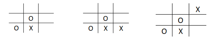
• Once the state is known, the bot must take an action in a way it considers to be optimum to win the game (policy)
• This move will result in a new scenario with new combinations of O’s and X’s which is a new state and a numerical reward will be given based on the quality of move with the goal of winning the game (cumulative reward)

For more clarity on the aforementioned reward, let us consider a match between bots O and X:

Consider the following situation encountered in tic-tac-toe:

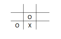
If bot X puts X in the bottom right position for example, it results in the following situation:

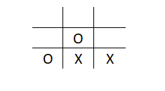
Bot O would be rejoicing (Yes! They are programmed to show emotions) as it can win the match with just one move. Now, we need to teach X not to do this again. So we give a negative reward or punishment to reinforce the correct behaviour in the next trial. We say that this action in the given state would correspond to a negative reward and should not be considered as an optimal action in this situation.

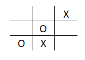
Similarly, a positive reward would be conferred to X if it stops O from winning in the next move:

Introduction to Markov Decision Process

Now that we understand the basic terminology, let’s talk about formalising this whole process using a concept called a Markov Decision Process or MDP.

A Markov Decision Process (MDP) model contains:

• A set of possible world states S
• A set of possible actions A
• A real valued reward function R(s,a)
• A description T of each action’s effects in each state

Now, let us understand the markov or ‘memoryless’ property.

Any random process in which the probability of being in a given state depends only on the previous state, is a markov process.

In other words, in the markov decision process setup, the environment’s response at time t+1 depends only on the state and action representations at time t, and is independent of whatever happened in the past.

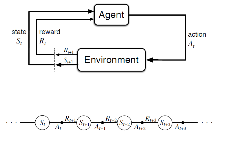
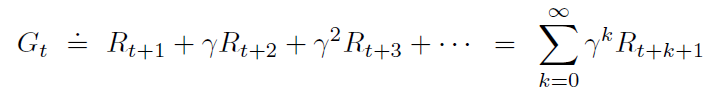
The above diagram clearly illustrates the iteration at each time step wherein the agent receives a reward R_t+1 and ends up in state S_t+1 based on its action A_t at a particular state S_t. The overall goal for the agent is to maximise the cumulative reward it receives in the long run. Total reward at any time instant t is given by:

where T is the final time step of the episode. In the above equation, we see that all future rewards have equal weight which might not be desirable. That’s where an additional concept of discounting comes into the picture. Basically, we define γ as a discounting factor and each reward after the immediate reward is discounted by this factor as follows:

For discount factor < 1, the rewards further in the future are getting diminished. This can be understood as a tuning parameter which can be changed based on how much one wants to consider the long term (γ close to 1) or short term (γ close to 0).

State Value Function: How good it is to be in a given state?

Can we use the reward function defined at each time step to define how good it is, to be in a given state for a given policy? The value function denoted as v(s) under a policy π represents how good a state is for an agent to be in. In other words, what is the average reward that the agent will get starting from the current state under policy π?

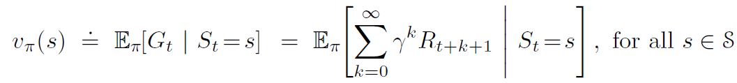
E in the above equation represents the expected reward at each state if the agent follows policy π and S represents the set of all possible states.

Policy, as discussed earlier, is the mapping of probabilities of taking each possible action at each state (π(a/s)). The policy might also be deterministic when it tells you exactly what to do at each state and does not give probabilities.

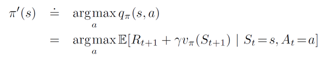
Now, it’s only intuitive that ‘the optimum policy’ can be reached if the value function is maximised for each state. This optimal policy is then given by:

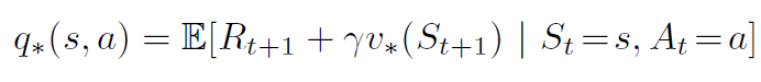
State-Action Value Function: How good an action is at a particular state?

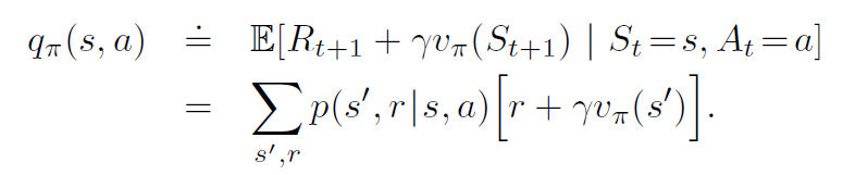
The above value function only characterizes a state. Can we also know how good an action is at a particular state? A state-action value function, which is also called the q-value, does exactly that. We define the value of action a, in state s, under a policy π, as:

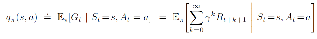
This is the expected return the agent will get if it takes action At at time t, given state St, and thereafter follows policy π.

Bellman Expectation Equation: The value information from successor states is being transferred back to the current state

Bellman was an applied mathematician who derived equations that help to solve an Markov Decision Process.

Let’s go back to the state value function v and state-action value function q. Unroll the value function equation to get:

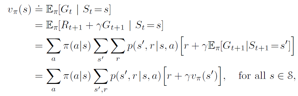
In this equation, we have the value function for a given policy π represented in terms of the value function of the next state.

Choose an action a, with probability π(a/s) at the state s, which leads to state s’ with prob p(s’/s,a). This gives a reward [r + γ*v_π(s)] as given in the square bracket above.

This is called the Bellman Expectation Equation. The value information from successor states is being transferred back to the current state, and this can be represented efficiently by something called a backup diagram as shown below.

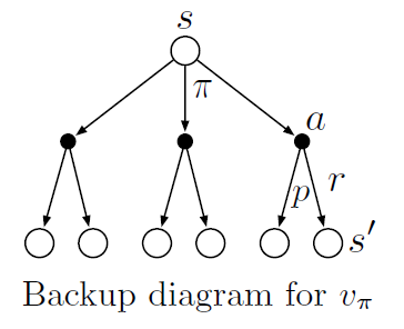
The Bellman expectation equation averages over all the possibilities, weighting each by its probability of occurring. It states that the value of the start state must equal the (discounted) value of the expected next state, plus the reward expected along the way.

We have n (number of states) linear equations with unique solution to solve for each state s.

Bellman Optimality Equation: Find the optimal policy

The goal here is to find the optimal policy, which when followed by the agent gets the maximum cumulative reward. In other words, find a policy π, such that for no other π can the agent get a better expected return. We want to find a policy which achieves maximum value for each state.

Note that we might not get a unique policy, as under any situation there can be 2 or more paths that have the same return and are still optimal.

Optimal value function can be obtained by finding the action a which will lead to the maximum of q*. This is called the bellman optimality equation for v*.

Intuitively, the Bellman optimality equation says that the value of each state under an optimal policy must be the return the agent gets when it follows the best action as given by the optimal policy. For optimal policy π*, the optimal value function is given by:

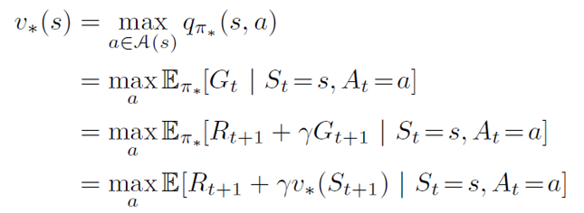
Given a value function q*, we can recover an optimum policy as follows:

The value function for optimal policy can be solved through a non-linear system of equations. We can can solve these efficiently using iterative methods that fall under the umbrella of dynamic programming.

Dynamic Programming

Dynamic programming algorithms solve a category of problems called planning problems. Herein given the complete model and specifications of the environment (MDP), we can successfully find an optimal policy for the agent to follow. It contains two main steps

Break the problem into subproblems and solve it. Solutions to subproblems are cached or stored for reuse to find an overall optimal solution to the problem at hand.

To solve a given MDP, the solution must have the components to:

1. Find out how good an arbitrary policy isFind out the optimal policy for the given MDP

Policy Evaluation: Find out how good a policy is?

Policy evaluation answers the question of how good a policy is. Given an MDP and an arbitrary policy π, we will compute the state-value function. This is called policy evaluation in the DP literature. The idea is to turn bellman expectation equation discussed earlier to an update.

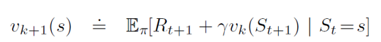
To produce each successive approximation vk+1 from vk, iterative policy evaluation applies the same operation to each state s. It replaces the old value of s with a new value obtained from the old values of the successor states of s, and the expected immediate rewards, along all the one-step transitions possible under the policy being evaluated, until it converges to the true value function of a given policy π.

Example of GridWorld

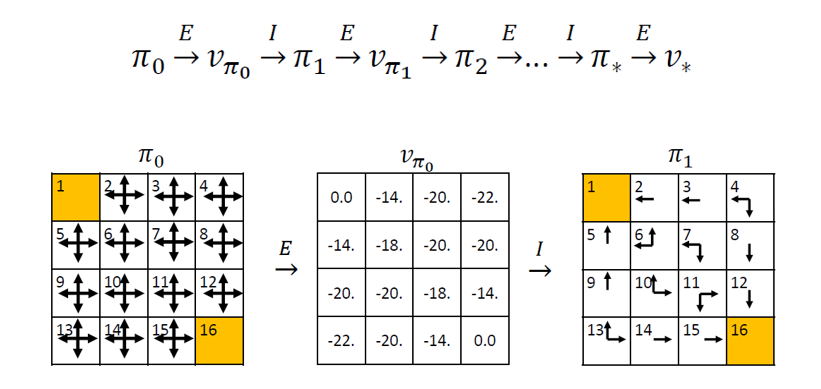
Let us understand policy evaluation using the very popular example of Gridworld.

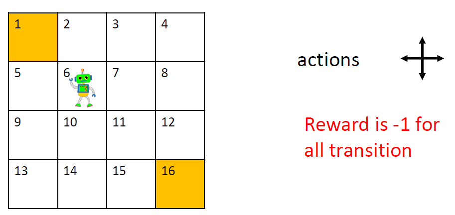
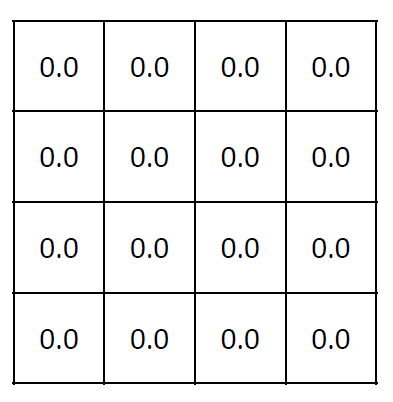
A bot is required to traverse a grid of 4×4 dimensions to reach its goal (1 or 16). Each step is associated with a reward of -1. There are 2 terminal states here: 1 and 16 and 14 non-terminal states given by [2,3,….,15]. Consider a random policy for which, at every state, the probability of every action {up, down, left, right} is equal to 0.25. We will start with initialising v₀ for the random policy to all 0s.

This is definitely not very useful. Let’s calculate v₂ for all the states of 6:

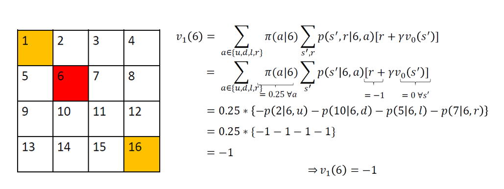
Similarly, for all non-terminal states, v₁(s) = -1.

For terminal states p(s’/s,a) = 0 and hence v_k(1) = v_k(16) = 0 for all k. So v₁ for the random policy is given by:

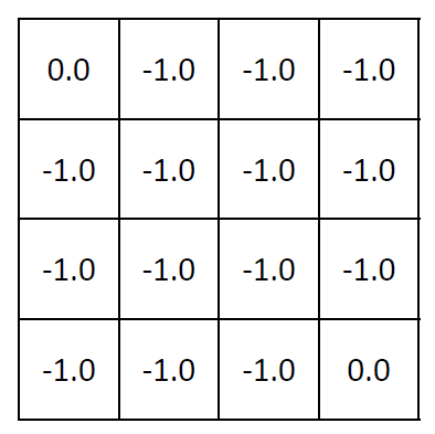
Now, for v₂(s) we are assuming γ or the discounting factor to be 1:

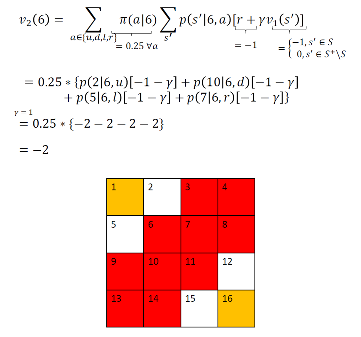
As you can see, all the states marked in red in the above diagram are identical to 6 for the purpose of calculating the value function. Hence, for all these states, v₂(s) = -2.

For all the remaining states, i.e., 2, 5, 12 and 15, v₂ can be calculated as follows:

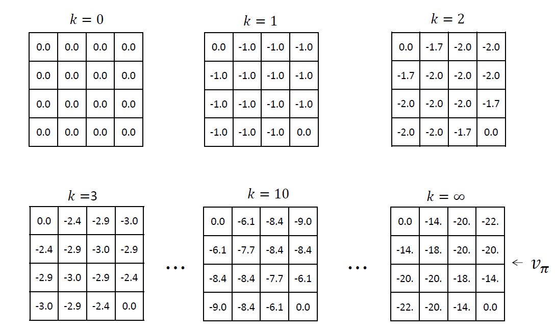
If we repeat this step several times, we get v_π:

Policy Improvement: Improve an arbitrary policy

Using policy evaluation we have determined the value function v for an arbitrary policy π. We know how good our current policy is. Now for some state s, we want to understand what is the impact of taking an action a that does not pertain to policy π.  Let’s say we select a in s, and after that we follow the original policy π. The value of this way of behaving is represented as:

If this happens to be greater than the value function v_π(s), it implies that the new policy π’ would be better to take. We do this iteratively for all states to find the best policy. Note that in this case, the agent would be following a greedy policy in the sense that it is looking only one step ahead.

Let’s get back to our example of gridworld. Using v_π, the value function obtained for random policy π, we can improve upon π by following the path of highest value (as shown in the figure below). We start with an arbitrary policy, and for each state one step look-ahead is done to find the action leading to the state with the highest value. This is done successively for each state.

As shown below for state 2, the optimal action is left which leads to the terminal state having a value . This is the highest among all the next states (0,-18,-20). This is repeated for all states to find the new policy.

Overall, after the policy improvement step using v_π, we get the new policy π’:

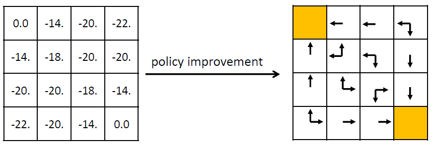
Looking at the new policy, it is clear that it’s much better than the random policy. However, we should calculate v_π’ using the policy evaluation technique we discussed earlier to verify this point and for better understanding.

Policy Iteration: Policy Evaluation + Policy Improvement

Once the policy has been improved using v_π to yield a better policy π’, we can then compute v_π’ to improve it further to π’’. Repeated iterations are done to converge approximately to the true value function for a given policy π (policy evaluation). Improving the policy as described in the policy improvement section is called policy iteration.

In this way, the new policy is sure to be an improvement over the previous one and given enough iterations, it will return the optimal policy. This sounds amazing but there is a drawback – each iteration in policy iteration itself includes another iteration of policy evaluation that may require multiple sweeps through all the states. Value iteration technique discussed in the next section provides a possible solution to this.

Value Iteration

We saw in the gridworld example that at around k = 10, we were already in a position to find the optimal policy. So, instead of waiting for the policy evaluation step to converge exactly to the value function v_π, we could stop earlier.

We can also get the optimal policy with just 1 step of policy evaluation followed by updating the value function repeatedly (but this time with the updates derived from bellman optimality equation). Let’s see how this is done as a simple backup operation:

This is identical to the bellman update in policy evaluation, with the difference being that we are taking the maximum over all actions. Once the updates are small enough, we can take the value function obtained as final and estimate the optimal policy corresponding to that.

Some important points related to DP:

1. 1. DP can only be used if the model of the environment is known.
   2. Has a very high computational expense, i.e., it does not scale well as the number of states increase to a large number. An alternative called asynchronous dynamic programming helps to resolve this issue to some extent.

DP in action: Finding optimal policy for Frozen Lake environment using Python

It is of utmost importance to first have a defined environment in order to test any kind of policy for solving an MDP efficiently. Thankfully, OpenAI, a non profit research organization provides a large number of environments to test and play with various reinforcement learning algorithms. To illustrate dynamic programming here, we will use it to navigate the Frozen Lake environment.

Frozen Lake Environment

The agent controls the movement of a character in a grid world. Some tiles of the grid are walkable, and others lead to the agent falling into the water. Additionally, the movement direction of the agent is uncertain and only partially depends on the chosen direction. The agent is rewarded for finding a walkable path to a goal tile.

The surface is described using a grid like the following:

(S: starting point, safe),  (F: frozen surface, safe), (H: hole, fall to your doom), (G: goal)

The idea is to reach the goal from the starting point by walking only on frozen surface and avoiding all the holes. Installation details and documentation is available at this link.

Once gym library is installed, you can just open a jupyter notebook to get started.

import gym
import numpy as np
env = gym.make('FrozenLake-v0')

Now, the env variable contains all the information regarding the frozen lake environment. Before we move on, we need to understand what an episode is. An episode represents a trial by the agent in its pursuit to reach the goal. An episode ends once the agent reaches a terminal state which in this case is either a hole or the goal.

Policy Iteration in python

Description of parameters for policy iteration function

policy: 2D array of a size n(S) x n(A), each cell represents a probability of taking action a in state s.

environment: Initialized OpenAI gym environment object

discount_factor: MDP discount factor

theta: A threshold of a value function change. Once the update to value function is below this number

max_iterations: Maximum number of iterations to avoid letting the program run indefinitely

This function will return a vector of size nS, which represent a value function for each state.

Let’s start with the policy evaluation step. The objective is to converge to the true value function for a given policy π. We will define a function that returns the required value function.

def policy_evaluation(policy, environment, discount_factor=1.0, theta=1e-9, max_iterations=1e9):
    """
    Evaluate a policy given an environment.

    Parameters:
    policy: The policy to evaluate, a 2D array where each state maps to a list of action probabilities.
    environment: The environment to evaluate against, containing transition probabilities and rewards.
    discount_factor: The discount factor for future rewards.
    theta: A threshold for the value function change to determine convergence.
    max_iterations: The maximum number of iterations to perform.

    Returns:
    V: The value function for the policy.
    """
    # Initialize the value function for each state to zero
    V = np.zeros(environment.nS)
    # Number of evaluation iterations
    evaluation_iterations = 1

    for i in range(int(max_iterations)):
        # Initialize a change of value function as zero
        delta = 0

        # Iterate through each state
        for state in range(environment.nS):
            # Initialize a new value of the current state
            v = 0

            # Try all possible actions which can be taken from this state
            for action, action_probability in enumerate(policy[state]):
                # Check how good the next state will be
                for state_probability, next_state, reward, terminated in environment.P[state][action]:
                    # Calculate the expected value
                    v += action_probability * state_probability * (reward + discount_factor * V[next_state])

            # Calculate the absolute change of value function
            delta = max(delta, np.abs(V[state] - v))
            # Update value function
            V[state] = v

        evaluation_iterations += 1

        # Terminate if value change is insignificant
        if delta < theta:
            print(f'Policy evaluated in {evaluation_iterations} iterations.')
            return V

    print(f'Maximum iterations reached. Policy evaluation terminated after {evaluation_iterations} iterations.')
    return V

Now coming to the policy improvement part of the policy iteration algorithm. We need a helper function that does one step lookahead to calculate the state-value function. This will return an array of length nA containing expected value of each action

def one_step_lookahead(environment, state, V, discount_factor):
        action_values = np.zeros(environment.nA)
        for action in range(environment.nA):
                for probability, next_state, reward, terminated in environment.P[state][action]:
                        action_values[action] += probability * (reward + discount_factor * V[next_state])
        return action_values

Now, the overall policy iteration would be as described below. This will return a tuple (policy,V) which is the optimal policy matrix and value function for each state.

def policy_iteration(environment, discount_factor=1.0, max_iterations=1e9):
        # Start with a random policy
        #num states x num actions / num actions
        policy = np.ones([environment.nS, environment.nA]) / environment.nA
        # Initialize counter of evaluated policies
        evaluated_policies = 1
        # Repeat until convergence or critical number of iterations reached
        for i in range(int(max_iterations)):
                stable_policy = True
                # Evaluate current policy
                V = policy_evaluation(policy, environment, discount_factor=discount_factor)
                # Go through each state and try to improve actions that were taken (policy Improvement)
                for state in range(environment.nS):
                        # Choose the best action in a current state under current policy
                        current_action = np.argmax(policy[state])
                        # Look one step ahead and evaluate if current action is optimal
                        # We will try every possible action in a current state
                        action_value = one_step_lookahead(environment, state, V, discount_factor)
                        # Select a better action
                        best_action = np.argmax(action_value)
                        # If action didn't change
                        if current_action != best_action:
                                stable_policy = True
                                # Greedy policy update
                                policy[state] = np.eye(environment.nA)[best_action]
                evaluated_policies += 1
                # If the algorithm converged and policy is not changing anymore, then return final policy and value function
                if stable_policy:
                        print(f'Evaluated {evaluated_policies} policies.')
                        return policy, V

Value Iteration in python

The parameters are defined in the same manner for value iteration. The value iteration algorithm can be similarly coded:

def value_iteration(environment, discount_factor=1.0, theta=1e-9, max_iterations=1e9):
        # Initialize state-value function with zeros for each environment state
        V = np.zeros(environment.nS)
        for i in range(int(max_iterationsations)):
                # Early stopping condition
                delta = 0
                # Update each state
                for state in range(environment.nS):
                        # Do a one-step lookahead to calculate state-action values
                        action_value = one_step_lookahead(environment, state, V, discount_factor)
                        # Select best action to perform based on the highest state-action value
                        best_action_value = np.max(action_value)
                        # Calculate change in value
                        delta = max(delta, np.abs(V[state] - best_action_value))
                        # Update the value function for current state
                        V[state] = best_action_value
                        # Check if we can stop
                if delta < theta:
                        print(f'Value-iteration converged at iteration#{i}.')
                        break

        # Create a deterministic policy using the optimal value function
        policy = np.zeros([environment.nS, environment.nA])
        for state in range(environment.nS):
                # One step lookahead to find the best action for this state
                action_value = one_step_lookahead(environment, state, V, discount_factor)
                # Select best action based on the highest state-action value
                best_action = np.argmax(action_value)
                # Update the policy to perform a better action at a current state
                policy[state, best_action] = 1.0
        return policy, V

Finally, let’s compare both methods to look at which of them works better in a practical setting. To do this, we will try to learn the optimal policy for the frozen lake environment using both techniques described above. Later, we will check which technique performed better based on the average return after 10,000 episodes.

def play_episodes(environment, n_episodes, policy):
        wins = 0
        total_reward = 0
        for episode in range(n_episodes):
                terminated = False
                state = environment.reset()
                while not terminated:
                        # Select best action to perform in a current state
                        action = np.argmax(policy[state])
                        # Perform an action an observe how environment acted in response
                        next_state, reward, terminated, info = environment.step(action)
                        # Summarize total reward
                        total_reward += reward
                        # Update current state
                        state = next_state
                        # Calculate number of wins over episodes
                        if terminated and reward == 1.0:
                                wins += 1
        average_reward = total_reward / n_episodes
        return wins, total_reward, average_reward

# Number of episodes to play
n_episodes = 10000
# Functions to find best policy
solvers = [('Policy Iteration', policy_iteration),
           ('Value Iteration', value_iteration)]
for iteration_name, iteration_func in solvers:
        # Load a Frozen Lake environment
        environment = gym.make('FrozenLake-v0')
        # Search for an optimal policy using policy iteration
        policy, V = iteration_func(environment.env)
        # Apply best policy to the real environment
        wins, total_reward, average_reward = play_episodes(environment, n_episodes, policy)
        print(f'{iteration_name} :: number of wins over {n_episodes} episodes = {wins}')
        print(f'{iteration_name} :: average reward over {n_episodes} episodes = {average_reward} \n\n')

Output:

We observe that value iteration has a better average reward and higher number of wins when it is run for 10,000 episodes.

What is the difference between dynamic programming and reinforcement learning?

Dynamic programming (DP) and reinforcement learning (RL) are both powerful tools in computer science for solving problems involving decision-making and sequential actions, but they approach the problem in fundamentally different ways. Temporal difference learning is a key concept within reinforcement learning. Here’s a breakdown of the key differences:

Understanding of the Surroundings:

• Dynamic Programming (DP): Considers the environment to be a perfect model. This implies that DP is aware of the precise ramifications (rewards and transitions) of every decision made in every state space.
• Reinforcement Learning (RL): Doesn’t need an ideal model. Through interacting with its surroundings and getting rewarded for its efforts, RL learns by making mistakes and learning from them.

Choosing the Best Course of Action:

• DP: Finds the optimal control or best course of action to maximize the overall reward using a deterministic methodology.
• RL: Adopts a more investigative strategy. It gains experience by making mistakes, and while the best answer it comes up with might not be optimal, it’s still good enough.

End Notes

In this article, we became familiar with model based planning using dynamic programming, which given all specifications of an environment, can find the best policy to take. I want to particularly mention the brilliant book on RL by Sutton and Barto which is a bible for this technique and encourage people to refer it. More importantly, you have taken the first step towards mastering reinforcement learning. Stay tuned for more articles covering different algorithms within this exciting domain.This article will help you understand full concepts of approximate dynamic programming and having transition probabilities to make these programming a dynamic programming methods.

Ankit Choudhary

IIT Bombay Graduate with a Masters and Bachelors in Electrical Engineering. I have previously worked as a lead decision scientist for Indian National Congress deploying statistical models (Segmentation, K-Nearest Neighbours) to help party leadership/Team make data-driven decisions. My interest lies in putting data in heart of business for data-driven decision making.