Introduction
The ability to predict what comes next in a sequence is fascinating. It’s one of the reasons I became interested in data science! Interestingly – human mind is really good at it, but that is not the case with machines. Given a mysterious plot in a book, the human brain will start creating outcomes. But, how to teach machines to do something similar?
Thanks to Deep Learning – we can do lot more today than what was possible a few years back. The ability to work with sequence data, like music lyrics, sentence translation, understanding reviews or building chatbots – all this is now possible thanks to sequence modeling.
And that’s what we will learn in this article. Since this is part of our deeplearning.ai specialization series, I expect that the reader will be aware of certain concepts. In case you haven’t yet gone through the previous articles or just need a quick refresher, here are the links:
-
- An Introductory Guide to Deep Learning and Neural Networks (Notes from deeplearning.ai Course #1)
- Improving Neural Networks – Hyperparameter Tuning, Regularization, and More (deeplearning.ai Course #2)
- A Comprehensive Tutorial to learn Convolutional Neural Networks from Scratch (deeplearning.ai Course #4)
In this final part, we will see how sequence models can be applied in different real-world applications like sentiment classification, image captioning, and many other scenarios.
Table of Contents
- Course Structure
- Course 5: Sequence Models
- Module 1: Recurrent Neural Networks (RNNs)
- Module 2: Natural Language Processing (NLP) and Word Embeddings
- Introduction to Word Embeddings
- Learning Word Embeddings: Word2vec & GloVe
- Applications using Word Embeddings
- Module 3: Sequence models & Attention mechanism
Course Structure
We have covered quite a lot in this series so far. Below is a quick recap of the concepts we have learned:
- Basics of deep learning and neural networks
- How a shallow and a deep neural network works
- How the performance of a deep neural network can be improved by hyperparameter tuning, regularization and optimization
- Working and implementations of Convolutional Neural Network from scratch
It’s time to turn our focus to sequence modeling. This course (officially labelled course #5 of the deep learning specialization taught by Andrew Ng) is divided into three modules:
- In module 1, we will learn about Recurrent Neural Networks and how they work. We will also cover GRUs and LSTMs in this module
- In module 2, our focus will be on Natural Language Processing and word embeddings. We will see how Word2Vec and GloVe frameworks can be used for learning word embeddings
- Finally, module 3 will cover the concept of Attention models. We will see how to translate big and complex sentences from one language to another
Ready? Let’s jump into module 1!
Course 5: Sequence Models
Module 1: Recurrent Neural Networks
The objectives behind the first module of course 5 are:
- To learn what recurrent neural networks (RNNs) are
- To learn several variants including LSTMs, GRUs and Bidirectional RNNs
Don’t worry if these abbreviations sound daunting – we’ll clear them up in no time.
But first, why sequence models?
To answer this question, I’ll show you a few examples where sequence models are used in real-world scenarios.
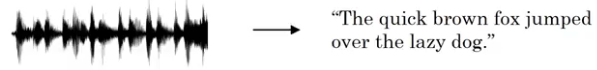
Speech recognition:
Quite a common application these days (everyone with a smartphone will know about this). Here, the input is an audio clip and the model has to produce the text transcript. The audio is considered a sequence as it plays over time. Also, the transcript is a sequence of words.
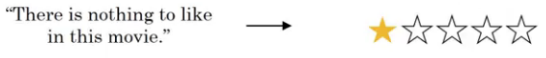
Sentiment Classification:
Another popular application of sequence models. We pass a text sentence as input and the model has to predict the sentiment of the sentence (positive, negative, angry, elated, etc.). The output can also be in the form of ratings or stars.
DNA sequence analysis:
Given a DNA sequence as input, we want our model to predict which part of the DNA belongs to which protein.
![]()
Machine Translation:
We input a sentence in one language, say French, and we want our model to convert it into another language, say English. Here, both the input and the output are sequences:

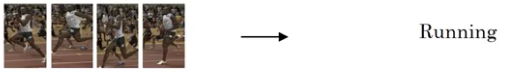
Video activity recognition:
This is actually a very upcoming (and current trending) use of sequence models. The model predicts what activity is going on in a given video. Here, the input is a sequence of frames.
Name entity recognition:
Definitely my favorite sequence model use case. As shown below, we pass a sentence as input and want our model to identify the people in that sentence:

Now before we go further, we need to discuss a few important notations that you will see throughout the article.
Notations we’ll use in this article
We represent a sentence with ‘X’. To understand further notifications, let’s take a sample sentence:
X : Harry and Hermione invented a new spell.
Now, to represent each word of the sentence, we use x<t>:
- x<1> = Harry
- x<2> = Hermoine, and so on
For the above sentence, the output will be:
y = 1 0 1 0 0 0 0
Here, 1 represents that the word represents a person’s name (and 0 means it’s anything but). Below are a few common notations we generally use:
- Tx = length of input sentence
- Ty = length of output sentence
- x(i) = ith training example
- x(i)<t> = tth training of ith training example
- Tx(i) = length of ith input sentence
At this point it’s fair to wonder – how do we represent n individual word in a sequence? Well, this is where we lean on a vocabulary, or a dictionary. This is a list of words that we use in our representations. A vocabulary might look like this:
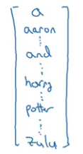
The size of the vocabulary might vary depending on the application. One potential way of making a vocabulary is by picking up the most frequently occurring words from the training set.
Now, suppose we want to represent the word ‘harry’ which is in the 4075th position in our vocabulary. We one-hot encode this vocabulary to represent ‘harry’:
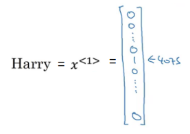
To generalize, x<t> is an one-hot encoded vector. We will put 1 in the 4075th position and all the remaining words will be represented as 0.
If the word is not in our vocabulary, we create an unknown <UNK> tag and add it in the vocabulary. As simple as that!
Recurrent Neural Network (RNN) Model
We use Recurrent Neural Networks to learn mapping from X to Y, when either X or Y, or both X and Y, are some sequences. But why can’t we just use a standard neural network for these sequence problems?
I’m glad you asked! Let me explain using an example. Suppose we build the below neural network:
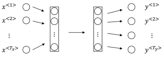
There are primarily two problems with this:
- Inputs and outputs do not have a fixed length, i.e., some input sentences can be of 10 words while others could be <> 10. The same is true for the eventual output
- We will not be able to share features learned across different positions of text if we use a standard neural network
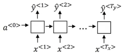
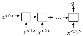
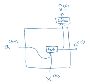
We need a representation that will help us to parse through different sentence lengths as well as reduce the number of parameters in the model. This is where we use a recurrent neural network. This is how a typical RNN looks like:
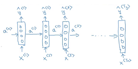
A RNN takes the first word (x<1>) and feeds it into a neural network layer which predicts an output (y’<1>). This process is repeated until the last time step x<Tx> which generates the last output y’<Ty>. This is the network where the number of words in input as well as the output are same.
The RNN scans through the data in a left to right sequence. Note that the parameters that the RNN uses for each time step are shared. We will have parameters shared between each input and hidden layer (Wax), every timestep (Waa) and between the hidden layer and the output (Wya).
So if we are making predictions for x<3>, we will also have information about x<1> and x<2>. A potential weakness of RNN is that it only takes information from the previous timesteps and not from the ones that come later. This problem can be solved using bi-directional RNNs which we will discuss later. For now, let’s look at forward propagation steps in a RNN model:
a<0> is a vector of all zeros and we calculate the further activations similar to that of a standard neural network:
- a<0> = 0
- a<1> = g(Waa * a<0> + Wax * x<1> + ba)
- y<1> = g’(Wya * a<1> + by)
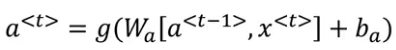
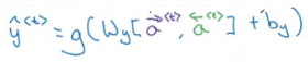
Similarly, we can calculate the output at each time step. The generalized form of these formulae can be written as:
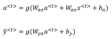
We can write these equations in an even more simpler way:
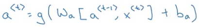
We horizontally stack Waa and Wya to get Wa. a<t-1> and x<t> are stacked vertically. Rather than carrying around 2 parameter matrices, we now have just 1 matrix. And that, in a nutshell, is how forward propagation works for recurrent neural networks.
Backpropagation through time
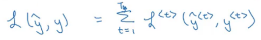
You might see this coming – the backpropagation steps work in the opposite direction to forward propagation. We have a loss function which we need to minimize in order to generate accurate predictions. The loss function is given by:

We calculate the loss at every timestep and finally sum all these losses to calculate the final loss for a sequence:
In forward propagation, we move from left to right, i.e., increasing the indices of time t. In backpropagation, we are going from right to left, i.e., going backward in time (hence the name backpropagation through time).
So far, we have seen scenarios where the length of input and output sequences was equal. But what if the length differs? Let’s see these different scenarios in the next section.
Different types of RNNs
We can have different types of RNNs to deal with use cases where the sequence length differs. These problems can be classified into the following categories:
Many-to-many
The name entity recognition examples we saw earlier fall under this category. We have a sequence of words, and for each word, we have to predict whether it is a name or not. The RNN architecture for such a problem looks like this:
For every input word, we predict a corresponding output word.
Many-to-one
Consider the sentiment classification problem. We pass a sentence to the model and it returns the sentiment or rating corresponding to that sentence. This is a many-to-one problem where the input sequence can have varied length, whereas there will only be a single output. The RNN architecture for such problems will look something like this:
Here, we get a single output at the end of the sentence.
One-to-many
Consider the example of music generation where we want to predict the lyrics using the music as input. In such scenarios, the input is just a single word (or a single integer), and the output can be of varied length. The RNN architecture for this type of problems looks like the below:

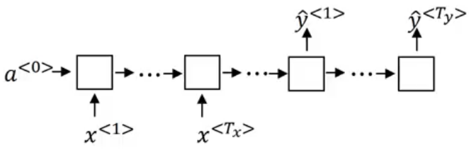
There is one more type of RNN which is popularly used in the industry. Consider the machine translation application where we take an input sentence in one language and translate it into another language. It is a many-to-many problem but the length of the input sequence might or might not be equal to the length of output sequence.
In such cases, we have an encoder part and a decoder part. The encoder part reads the input sentence and the decoder translates it to the output sentence:
Language model and sequence generation
Suppose we are building a speech recognition system and we hear the sentence “the apple and pear salad was delicious”. What will the model predict – “the apple and pair salad was delicious” or “the apple and pear salad was delicious”?
I would hope the second sentence! The speech recognition system picks this sentence by using a language model which predicts the probability of each sentence.
But how do we build a language model?
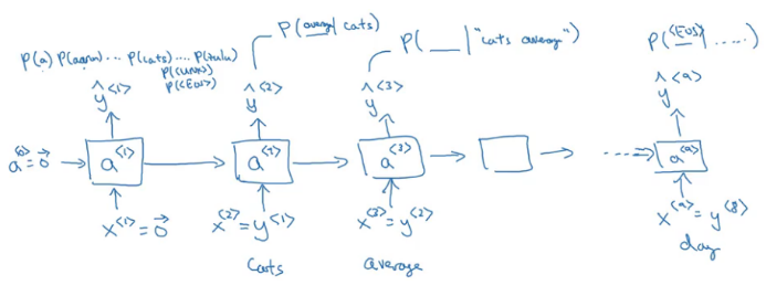
Suppose we have an input sentence:
Cats average 15 hours of sleep a day.
The steps to build a language model will be:
- Step 1 – Tokenize the input, i.e. create a dictionary
- Step 2 – Map these words to a one-hot encode vector. We can add <EOS> tag which represents the End Of Sentence
- Step 3 – Build an RNN model
We take the first input word and make a prediction for that. The output here tells us what is the probability of any word in the dictionary. The second output tells us the probability of the predicted word given the first input word:
Each step in our RNN model looks at some set of preceding words to predict the next word. There are various challenges associated with training an RNN model and we will discuss them in the next section.
Vanishing gradients with RNNs
One of the biggest problems with a recurrent neural network is that it runs into vanishing gradients. How? Consider the two sentences:
The cat, which already ate a bunch of food, was full.
The cat, which already ate a bunch of food, were full.
Which of the above two sentences is grammatically correct? It’s the first one (read it again in case you missed it!).
Basic RNNs are not good at capturing long term dependencies. This is because during backpropagation, gradients from an output y would have a hard time propagating back to affect the weights of earlier layers. So, in basic RNNs, the output is highly affected by inputs closer to that word.
If the gradients are exploding, we can clip them by setting a pre-defined threshold.
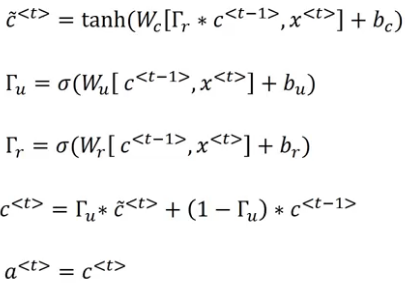
Gated Recurrent Units (GRUs)
GRUs are a modified form of RNNs. They are highly effective at capturing much longer range dependencies and also help with the vanishing gradient problem. The formula to calculate activation at timestep t is:
A hidden unit of RNN looks like the below image:
The inputs for a unit are the activations from the previous unit and the input word of that timestep. We calculate the activations and the output at that step. We add a memory cell to this RNN in order to remember the words present far away from the current word. Let’s look at the equations for GRU:
c<t> = a<t>
where c is a memory cell.
At every timestep, we overwrite the c<t> value as:
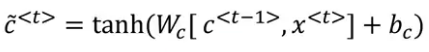
This acts as a candidate for updating the c<t> value. We also define an update gate which decides whether or not we update the memory cell. The equation for update gate is:
![]()
Notice that we are using sigmoid to calculate the update value. Hence, the output of update gate will always be between 0 and 1. We use the previous memory cell value and the update gate output to update the memory cell. The update equation for c<t> is given by:
![]()
When the gate value is 0, c<t> = c<t-1>, i.e., we do not update c<t>. When the gate value is 1, c<t> = c<t> and the value is updated. Let’s understand this mind-bending concept using an example:

We have the gate value as 1 when we are at the word cat. For all other words in the sequence, the gate value is 0 and hence the information of the cat will be carried till the word ‘was’. We expect the model to predict was in place of were.
This is how GRUs helps to memorize long term dependencies. Here is a visualization to help you understand the working of a GRU:
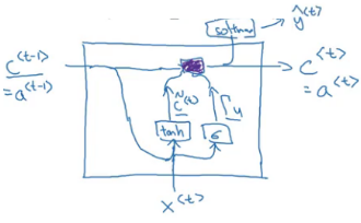
For every unit, we have three inputs : a<t-1>, c<t-1> and x<t> and three outputs : a<t>, c<t> and y(hat)<t>.
Long Short Term Memory (LSTM)
LSTMs are all the rage in deep learning these days. They might not have a lot of industry applications right now because of their complexity but trust me, they will very, very soon. It’s worth taking out time to learn this concept – it will come in handy in the future.
Now to understand LSTMs, let’s recall all the equations we saw for GRU:
We have just added one more gate while calculating the relevance for c<t> and this gate tells us how relevant c<t-1> is for updating c<t>. For GRUs, a<t> = c<t>.
LSTM is a more generalized and powerful version of GRU. The equation for LSTM is:
![]()
This is similar to that of GRU, right? We are just using a<t-1> instead of c<t-1>. We also have an update gate:
![]()
We also have a forget gate and an output gate in LSTM. The equations for these gates are similar to that of the update gate:
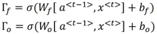
Finally, we update the c<t> value as:
![]()
And the activations for the next layer will be:
![]()
So which algorithm should you use – GRU or LSTM?
Each algorithm has it
s advantages. You’ll find that their accuracy varies depending on the kind of problem you’re trying to solve. The advantage with GRU is that it has a simpler architecture and hence we can build bigger models, but LSTM is more powerful and effective as it has 3 gates instead of 2.
Bidirectional RNN
The RNN architectures we have seen so far focus only on the previous information in a sequence. How awesome would it be if our model can take into account both the previous as well as the later information of the sequence while making predictions at a particular timestep?
Yes, that’s possible! Welcome to the world of bidirectional RNNs. But before I introduce you to what Bidirectional RNNs are and how they work, let’s first look at why we need them.
Consider the named entity recognition problem where we want to know whether a word in a sequence represents a person. We have the following example:
He said, “Teddy bears are on sale!”
If we feed this sentence to a simple RNN, the model will predict “Teddy” to be the name of a person. It just doesn’t take into account what comes after that word. We can fix this issue with the help of bidirectional RNNs.
Now suppose we have an input sequence of 4 words. A bidirectional RNN will look like:
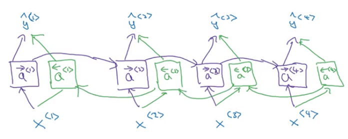
To calculate the output from a RNN unit, we use the following formula:
Similarly, we can have bidirectional GRUs and bidirectional LSTMs. One disadvantage of using bidirectional RNNs is that we have to look at the entire sequence of data before making any prediction. But the standard B-RNN algorithm is actually very effective for building and designing most NLP applications.
Deep RNNs
Remember what a deep neural network looks like?
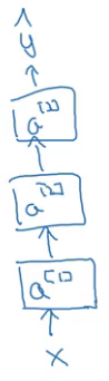
We have an input layer, some hidden layers and finally an output layer. A deep RNN also looks like this. We take a similar network and unroll that in time:
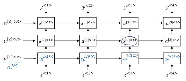
Here, the generalized notation for activations is given as:
a[l]<t> = activation of lth later at time t
Suppose we want to calculate a[2]<3> :
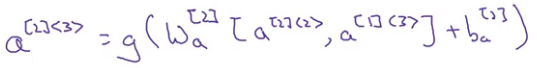
That’s it for deep RNNs. Take a deep breath, that was quite a handful to digest in one go. And now, time to move to module 2!
Module 2: Natural Language Processing & Word Embeddings
The objectives for studying the second module are:
- To learn natural language processing using deep learning techniques
- To understand how to use word vector representations and embedding layers
- To embellish our learning with a look at the various applications of NLP, like sentiment analysis, named entity recognition and machine translation
Part 1 – Introduction to Word Embeddings
Word Representation
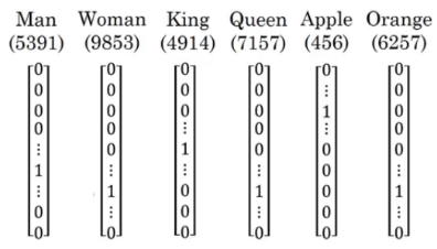
Up to this point, we have used a vocabulary to represent words:
![]()
To represent a single word, we created a one-hot vector:
Now, suppose we want our model to generalize between different words. We train the model on the following sentence:
I want a glass of Apple juice.
We have given “I want a glass of Apple” as the training sequence and “juice” as the target. We want our model to generalize the solution of, say:
I want a glass of Orange ____ .
Why won’t our previous vocabulary approach work? Because it lacks the flexibility to generalize. We will try to calculate the similarity between the vector representing the words Apple and Orange. We’ll inevitably get zero as output as the product of any two one-hot vectors is always zero.
Instead of having a one-hot vector for representations, what if we represent each word with a set of features? Check out this table:
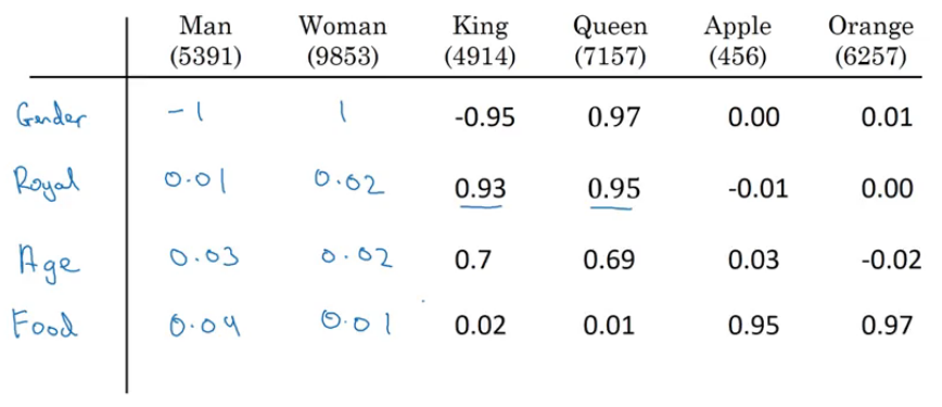 We can find similar words using this approach. Quite useful, isn’t it?
Say, we have 300 features for each word. So, for example, the word ‘Man’ will be represented by a 300 dimensional vector named e5391.
We can also use these representations for visualization purposes. Convert the 300 dimensional vector into a 2-d vector and then plot it. Quite a few algorithms exist for doing this but my favorite one is easily t-SNE.
Using word embeddings
Word embeddings really help us to generalize well when working with word representations.
Suppose you are performing a named entity recognition task and only have a few records in the training set. In such a case, you can either take pretrained word embeddings available online or create your own embeddings. These embeddings will have features for all the words in that vocabulary.
Here are the two primary steps for replacing one-hot encoded representations with word embeddings:
- Learn word embeddings from a large text corpus (or download pretrained word embeddings)
- Transfer these embeddings to a new task with a smaller training set
Next, we will look at the properties of word embeddings.
Properties of word embeddings
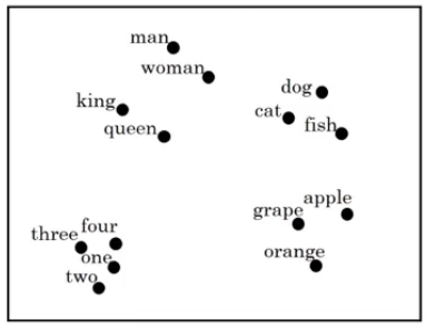
Suppose you get a question – “If Man is to Woman, then King is to?”. Most keen puzzle solvers will have seen these kind of questions before!
The likely answer to this question is Queen. But how will the model decide that? This is actually one of the most widely used examples to understand word embeddings. We have embeddings for Man, Woman, King and Queen. The embedding vector of Man will be similar to that of Woman and the embedding vector of King will be similar to that of Queen.
We can use the following equation:
eman – ewoman = eking – ?
Solving this gives us a 300 dimensional vector with a value equal to the embeddings of queen. We can use a similarity function to determine the similarity between two word embeddings as well. The similarity function is given by:
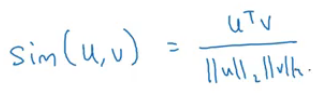
This is a cosine similarity. We can also use the Euclidean distance formula:
![]()
There are a few other different types of similarity measures which you’ll find in core recommendation systems.
Embedding matrix
We actually end up learning an embedding matrix when we implement a word embeddings algorithm. If we’re given a vocabulary of 10,000 words and each word has 300 features, the embedding matrix, represented as E, will look like this:
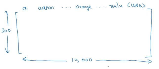
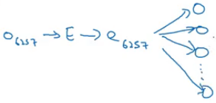
To find the embeddings of the word ‘orange’ which is at the 6257th position, we multiply the above embedding matrix with the one-hot vector of orange:
E . O6257 = e6257
The shape of E is (300, 10k), and of O is (10k, 1). Hence, the embedding vector e will be of the shape (300, 1).
Part 2 – Learning Word Embeddings: Word2Vec & GloVe
Learning Word Embeddings
Consider we are building a language model using a neural network. The input to the model is “I want a glass of orange” and we want the model to predict the next word.
We will first learn the embeddings of each of the words in the sequence using a pre trained word embedding matrix and then pass those embeddings to a neural network which will have a softmax classifier at the end to predict the next word.
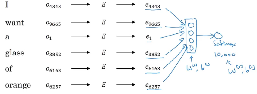
This is how the architecture will look like. In this example we have 6 input words, each word is represented by a 300 dimensional vector and hence the input of the sequence will be 6*300 = 1800 dimensional. The parameters for this model are:
- Embedding matrix (E)
- W[1], b[1]
- W[2], b[2]
We can reduce the number of input words, to decrease the input dimensions. We can say that we want our model to use previous 4 words only to make prediction. In this case the input will be 1200 dimensional. The input can also be referred as context and there can be various ways to select the context. Few possible ways are:
- Take last 4 words
- Take 4 words from left and 4 words from right
- Last 1 word
- We can also take one nearby word
This is how we can solve language modeling problem where we input the context and predict some target words. In the next section, we will look at how Word2Vec can be applied for learning word embeddings.
Word2Vec
It is a simple and more efficient way to learn word embeddings. Consider we have a sentence in our training set:
I want a glass of orange juice to go along with my cereal.
We use a skip gram model to pick a few context and target words. In this way we create a supervised learning problem where we have an input and its corresponding output. For context, instead of having only last 4 words or last 1 word, we randomly pick a word to be the context word and then randomly pick another word within some window (say 5 to the left and right) and set that as the target word. Some of the possible context – target pairs could be:
| Context | Target |
| orange | juice |
| orange | glass |
| orange | my |
These are only few pairs, we can have many more pairs as well. Below are the details of the model:
Vocab size = 10,000k
Now, we want to learn a mapping from some context (c) to some target (t). This is how we do the mapping:
Oc -> E -> ec -> softmax -> y(hat)
Here, ec = E.Oc
Here softmax is calculating the probability of getting the target word (t) as output given the context word (c).
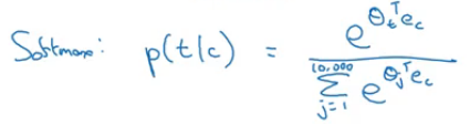
Finally, we calculate the loss as:
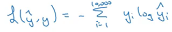
Using a softmax function creates a couple of problems to the algorithm, one of them is computational cost. Everytime we calculate the probability:
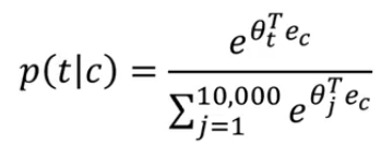
We have to carry out the sum over all 10,000 words in the vocabulary. If we use a larger vocabulary of say 100,000 words or even more the computation gets really slow. Few solutions to this problem are:
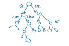
Using a hierarchical softmax classifier. So, instead of classifying some word into 10,000 categories in one go, we first classify it into either first 5000 categories or later 5000 categories, and so on. In this way we do not have to compute the sum over all 10,000 words every time. The flow of hierarchical softmax classifier looks like:
One question that might arise in your mind is how to choose the context c? One way could be to sample the context word at random. The problem with random sampling is that the common words like is, the will appear more frequently whereas the unique words like orange, apple might not even appear once. So, we try to choose a method which gives more weightage to less frequent words and less weightage to more frequent words.
In the next section we will see a technique that helps us to reduce the computation cost and learn much better word embeddings.
Negative Sampling
In the skip gram models, as we have seen earlier, we map context words to target words which allows us to learn word embeddings. One downside of that model was high computational cost due to softmax. Consider the same example that we took earlier:
I want a glass of orange juice to go along with my cereal.
What negative sampling will do is, it creates a new supervised learning problem, where given a pair of words say “orange” and “juice”, we will predict whether it is a context-target pair? For the above example, the new supervised learning problem will look like:
| Context (c) | Word (t) | Target (y) |
| orange | juice | 1 |
| orange | king | 0 |
| orange | book | 0 |
| orange | the | 0 |
Since orange-juice is a context-target pair, we set the Target value as 1, whereas, orange-king is not a pair for above example, and hence Target is 0. These 0 values represent that it is a negative sample. We now apply a logistic regression to calculate the probability of whether the pair is a context-target pair or not. The probability is given by:
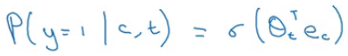
We can have k pair of words for training the model. k can range between 5-20 for smaller dataset while for larger dataset, we choose smaller k (2-5). So, if we build a neural network and the input is orange (one hot vector of orange):
We will have 10,000 possible classification problems each corresponding to different words from the vocabulary. So, this network will tell all the possible target words corresponding to the context word orange. Here, instead of having one giant 10,000 way softmax, which is computationally very slow, we have 10,000 binary classification problems which is comparatively faster as compared to the softmax.
Context word is chosen from the sequence and once it is chosen, we randomly pick another word from the sequence to be a positive sample and then pick few of the other random words from the vocabulary as negative samples. In this way, we can learn word embeddings using simple binary classification problems. Next we will see even simpler algorithm for learning word embeddings.
GloVe word vectors
We will work on the same example:
I want a glass of orange juice to go along with my cereal.
Previously, we were sampling pairs of words (context and target) by picking two words that appears in close proximity to each other from our text corpus. GloVe or Global Vectors for word representation makes it more explicit. Let’s say:
Xij = number of times i appears in context of j
Here, i is similar to the target (t) and j is similar to the context (c). GloVe minimizes the following:
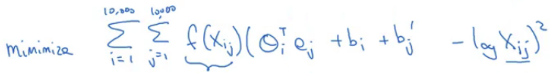
Here, f(Xij) is the weighing term. It gives less weightage to more frequent words (such as stop words like this, is, of, a, ..) and more weightage to less frequent words. Also, f(Xij) = 0 when (Xij) = 0. It has been found that minimizing the above equation finally leads to a good word embeddings. Now, we have seen many algorithms for learning word embeddings. Next we will see the application using word embeddings.
Part 3 – Applications using Word Embeddings
Sentiment Classification
You must already be well aware of what sentiment classification is so I’ll make this quick. Check out the below table which contains some text and its corresponding sentiment:
| X (text) | y (sentiment) |
| The dessert is excellent. | **** |
| Service was quite slow. | ** |
| Good for a quick meal, but nothing special. | *** |
| Completely lacking in good taste | * |
The applications of sentiment classification are varied, diverse and HUGE. But In most cases you’ll encounter, the training doesn’t come labelled. This is where word embeddings come to the rescue. Let’s see how we can use word embeddings to build a sentiment classification model.
We have the input as: “The dessert is excellent”.
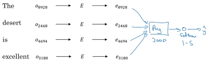
Here, E is the pretrained embedding matrix of, say, 100 billion words. We multiple the one-hot encoded vectors of each word with the embedding matrix to get the word representations. Next, we sum up all these embeddings and apply a softmax classifier to decide what should be the rating of that review.
It only takes the mean of all the words, so if the review is negative but it has more positive words, then the model might give it a higher rating. Not a great idea. So instead of just summing up the embedding to get the output, we can use an RNN for sentiment classification.
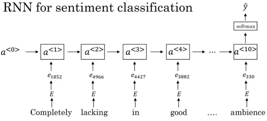
This is a many-to-one problem where we have a sequence of inputs and a single output. You are now well equipped to solve this problem. 🙂
Module 3: Sequence Models & Attention Mechanism
Welcome to the final module of the series! Below are the two objectives we will primarily achieve in this module:
- Understanding the attention mechanism
- To understand where the model should focus its attention given an input sequence
Basic Models
I’m going to keep this section industry relevant, so we’ll cover models which are useful for applications like machine translation, speech recognition, etc. Consider this example – we are tasked with building a sequence-to-sequence model where we want to input a French sentence and translate it into English. The problem will look like:
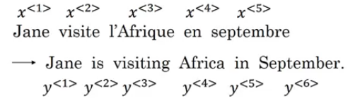
Here x<1>, x<2> are the inputs and y<1>, Y<2> are outputs. To build a model for this, we have an encoder part which takes an input sequence. The encoder is built as an RNN, or LSTM, or GRU. After the encoder part, we build a decoder network which takes the encoding output as input and is trained to generate the translation of the sentence.
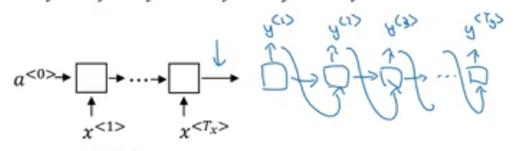
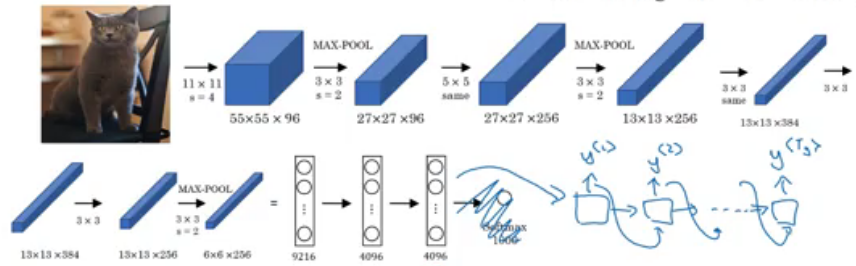
This network is popularly used for Image Captioning as well. As input, we have the image’s features (generated using a convolutional neural network).
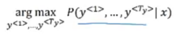
Picking the most likely sentence
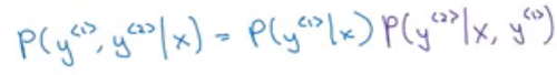
The decoder model of a machine translation system is quite similar to that of a language model. But there is one key difference between the two. In a language model, we start with a vector of all zeros, whereas in machine translation, we have an encoder network:
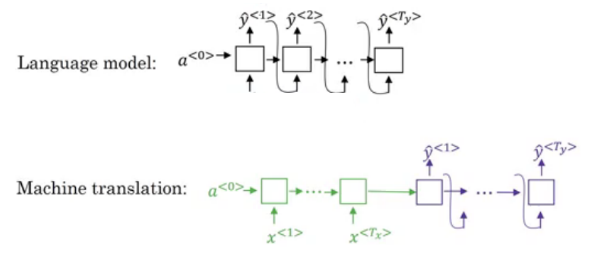
The encoder part of the machine translation model is a conditional language model where we are calculating the probability of outputs given an input:
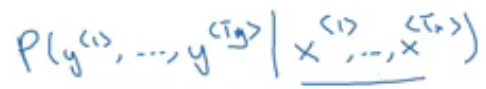
Now, for the input sentence:
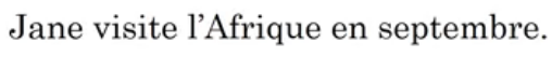
We can have multiple translations like:
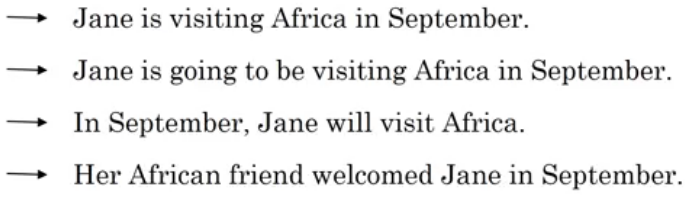
We want the best translation out of all the above sentences.
The good news? There is an algorithm that helps us choose the most likely translation.
Beam Search
This is one of the most commonly used algorithms for generating the most likely translations. The algorithm can be understood using the below 3 steps:
Step 1: It picks the first translated word and calculates its probability:
![]()
Instead of just picking one word, we can set a bean width (B) to say B=3. It will pick the top 3 words that can possibly be the first translated word. These three words are then stored in the computer’s memory.
Step 2: Now, for each selected word in step 1, this algorithm calculates the probability of what the second word could be:
If the beam width is 3 and there are 10,000 words in the vocabulary, the total number of possible combinations will be 3 * 10,000 = 30,000. We evaluate all these 30,000 combinations and pick the top 3 combinations.
Step 3: We repeat this process until we get to the end of the sentence.
By adding one word at a time, beam search decides the most likely translation for any given sentence. Let’s look at some of the refinements we can do to beam search in order to make it more effective.
Refinements to Beam Search
Beam search maximizes this probability:
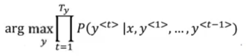
This probability is calculated by multiplying probabilities of different words. Since particular probabilities are very tiny numbers (between 0 and 1), if we multiply such small numbers multiple time, final output is very small which creates problem in computations. So, instead we can use the following formula to calculate the probabilities:
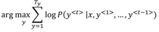
So, instead of maximizing the products, we maximize the log of a product. Even using this objective function, if the translated sentence has more words, their product will go down to more negative values, and hence we can normalize the function as:
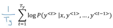
So, for all the sentences selected using beam search, we calculate this normalized log likelihood and then pick the sentence which gives the highest value. There is one more detail that I would like to share and it is how to decide the beam width B?
If the beam width is more, we will have better results but the algorithm will become slow. On the other hand, choosing smaller B will make the algorithm run faster but the results will not be accurate. There is no hard rule to choose beam width and it can vary according to the applications. We can try different values and then choose the one that gives the best results.
Error analysis in beam search
Beam search is an approximation algorithm which outputs the most likely translations based on the beam width. But it is not always necessary that it will generate the correct translation everytime. If we are not getting the correct translations, we have to analyse whether it is due to the beam search or our RNN model is causing problems. If we find that the beam search is causing the problem, we can increase the beam width and hopefully we will get better results. How to decide whether we should focus on improving the beam search or the model?
Suppose the actual translation is:
Jane visits Africa in September (y*)
And the translation that we got from the algorithm is:
Jane visited Africa last September (y(hat))
RNN will compute P(y* | x) and P(y(hat) | x)
Case 1: P(y* | x) > P(y(hat) | x)
This means beam search chose y(hat) but y* attains higher probability. So, beam search is at fault and we might consider increasing the beam width.
Case 2: P(y* | x) <= P(y(hat) | x)
This means that y* is better translation than y(hat) but RNN predicted the opposite. Here, RNN is at fault and we have to improve the model.
So, for each translation, we decide whether RNN is at fault or the beam search. Finally we figure out what fraction of errors are caused due to beam search vs RNN model and update either beam search or RNN model based on which one is more at fault. In this way we can improve the translations.
Attention Model
Up to this point, we have seen the encoder-decoder architecture for machine translation where one RNN reads the input and the other one outputs a sentence. But when we get very long sentences as input, it becomes very hard for the model to memorize the entire sentence.
What attention models do is they take small samples from the long sentence and translate them, then take another sample and translate them, and so on.
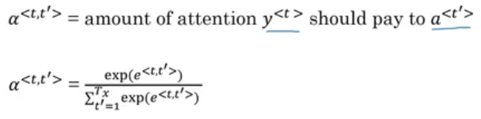
We use an alpha parameter to decide how much attention should be given to a particular input word while we generate the output.
⍺<1,2> = For generating the first word, how much attention should be given to the second input word
Let’s understand this with an example:
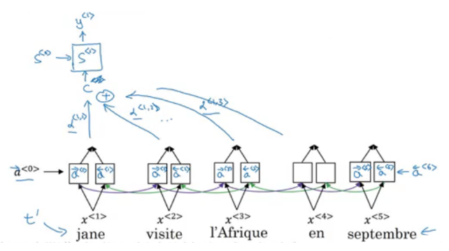
So, for generating the first output y<1>, we take attention weights for each word. This is how we compute the attention:
If we have Tx input words and Ty output words, then the total attention parameters will be Tx * Ty.
You might already have gathered this – Attention models are one of the most powerful ideas in deep learning.
End Notes
Sequence models are awesome, aren’t they? They have a ton of practical applications – we just need to know the right technique to use in specific situations. And my hope is that you will have learned those techniques in this guide.
Word embeddings are a great way to represent words and we saw how these word embeddings can be built and use. We have gone through different applications of word embeddings and finally we covered attention models as well which are one of the most powerful ideas for building sequence models.
If you have any query or feedback related to the article, feel free to share them in the comments section below. Looking forward to your responses!
Pulkit Sharma
12 May, 2020
My research interests lies in the field of Machine Learning and Deep Learning. Possess an enthusiasm for learning new skills and technologies.


Hi Pulkit, As Always, a good work .. Thanks for sharing such a wonderful article.. Please share your knowledge like that, so that we can learn something from you.
pretty interesting post
Glad you liked it jae!
How can you just take all of the deeplearning.ai course content and share it here on your website as your own? Have you taken permission from Andrew Ng?
Hi Anupam, These articles are my notes from deeplearning.ai courses. We have mentioned this in the headings of each article as well.
"Here, instead of having one giant 10,000 way softmax, which is computationally very slow, we have 10,000 binary classification problems which is comparatively very slow as compared to the softmax." - Do you mean comparitively fast? Are you advocating this as a solution for the softmax problem or not?
Hi Vinod, Thanks for pointing it out. 10000 binary classification problems are comparatively faster as compared to a single giant 10000 way softmax. I have also updated it in the article.