Introduction
Building that first model – isn’t that what we strive for in the deep learning field? That feeling of euphoria when we see our model running successfully is unparalleled. But the buck doesn’t stop there.
How can we improve the accuracy of the model? Is there any way to speed up the training process? These are critical questions to ask, whether you’re in a hackathon setting or working on a client project. And these aspects become even more prominent when you’ve built a deep neural network.

Features like hyperparameter tuning, regularization, batch normalization, etc. come to the fore during this process. This is part 2 of the deeplearning.ai course (deep learning specialization) taught by the great Andrew Ng. We saw the basics of neural networks and how to implement them in part 1, and I recommend going through that if you need a quick refresher.
In this article, we will explore the inner workings of these neural networks, including looking at how we can improve their performance and reduce the overall training time. These techniques have helped data scientists climb machine learning competition leaderboards (among other things) and earn top accolades. Yes, these concepts are invaluable!
Table of Contents
- Course Structure
- Course 2: Improving Deep Neural Networks: Hyperparameter tuning, Regularization and Optimization
- Module 1: Practical Aspects of Deep Learning
- Setting up your Machine Learning Application
- Regularizing your Neural Network
- Setting up your Optimization problem
- Module 2: Optimization Algorithms
- Module 3: Hyperparameter tuning, Batch Normalization and Programming Frameworks
- Hyperparameter tuning
- Batch Normalization
- Multi-class Classification
- Introduction to programming frameworks
- Module 1: Practical Aspects of Deep Learning
1. Course Structure
Part 1 of this series covered concepts like how both shallow and deep neural networks work, how to implement forward and backpropagation on single as well as multiple training examples, among other things. Now comes the question of how to tweak these neural networks in order to extract the maximum accuracy out of them.
Course 2, which we will see in this article, spans three modules:
- In module 1, we will be covering the practical aspects of deep learning. We will see how to split the training, validation and test sets from the given data. We will also be covering topics like regularization, dropout, normalization, etc. that help us make our model more efficient.
- In module 2, we will discuss the concept of a mini-batch gradient descent and a few more optimizers like Momentum, RMSprop, and ADAM.
- In the last module, we will see how different hyperparameters can be tuned to improve the model’s efficiency. We will also cover the concept of Batch Normalization and how to solve a multi-class classification challenge.
Course 2: Improving Deep Neural Networks: Hyperparameter tuning, Regularization and Optimization
Now that we know what all we’ll be covering in this comprehensive article, let’s get going!
Module 1: Practical Aspects of Deep Learning
The below pointers summarize what we can expect from this module:
- Recalling that different types of initializations lead to different results
- Recognizing the importance of initialization in complex neural networks
- Recognizing the difference between train/validation/test sets
- Diagnosing the bias and variance issues in our model
- Learning when and how to use regularization methods such as dropout or L2 regularization
- Understanding experimental issues in deep learning, such as Vanishing or Exploding gradients and how to deal with them
- Using gradient checking to verify the correctness of our backpropagation implementation
This module is fairly comprehensive, and is thus further divided into three parts:
- Part I: Setting up your Machine Learning Application
- Part II: Regularizing your Neural Network
- Part III: Setting up your Optimization Problem
Let’s walk through each part in detail.
Part I: Setting up your Machine Learning Application
Train / Dev / Test sets
While training a deep neural network, we are required to make a lot of decisions regarding the following hyperparameters:
- Number of hidden layers in the network
- Number of hidden units for each hidden layer
- Learning rate
- Activation function for different layers, etc.
There is no specified or pre-defined way of choosing these hyperparameters. The below is what we generally follow:
- Start with an idea, i.e. start with a certain number of hidden layers, certain learning rate, etc.
- Try the idea by coding it
- Experiment how well the idea has worked
- Refine the idea and iterate this process
Now how do we identify whether the idea is working? This is where the train / dev / test sets come into play. Suppose we have an entire dataset:![]()
We can divide this dataset into three different sets like: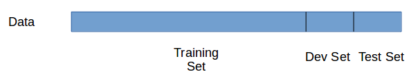
- Training Set: We train the model on the training data.
- Dev Set: After training the model, we check how well it performs on the dev set.
- Test Set: When we have a final model (i.e., the model that has performed well on both training as well as dev set), we evaluate it on the test set in order to get an unbiased estimate of how well our algorithm is doing.
There is still one question left after this – what should be the length of these training, dev and test sets? It’s actually a pretty critical aspect of any machine learning project, and will end up playing a big part in deciding how well the model performs. Let’s look at some traditional guidelines that experts follow to decide the length of each set:
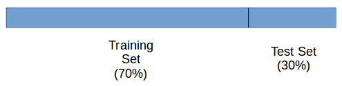
- In the previous era, when we had small datasets, the distribution of different sets was:
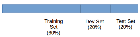
or just:
- As the availability of data has increased in recent years, we can use a huge slice of it for training the model:
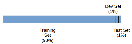
This is certainly one way of deciding the length of these different sets. This works fine most of the time, but indulge me and consider the following scenario:
Suppose we have scraped multiple images of cats from different sites, and also clicked a few images using our own camera. The distribution of both these types of images will be different, right? Now, we split the data in such a way that the training set contains all the scraped images, while the dev and test sets have all the camera images. In this case, the distribution of the training set will be different from the dev and test sets and hence, there’s a good chance we might not get good results.
In cases like these (different distributions), we can follow the following guidelines:
- Divide the training, dev and test sets in such a way that their distribution is similar
- Skip the test set and validate the model using the dev set only
We can also use these sets to look at the bias and variance of the model, These help us decide how well the model is fitting and performing.
Bias / Variance
Consider a dataset which gives us the below plot: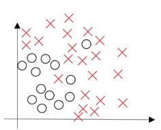
What will happen if we fit a straight line to classify the points into different classes? The model will under-fit and have a high bias. On the other hand, if we fit the data perfectly, i.e., all the points are classified into their respective class, we will have high variance (and overfitting). The right model fit is usually found between these two extremes: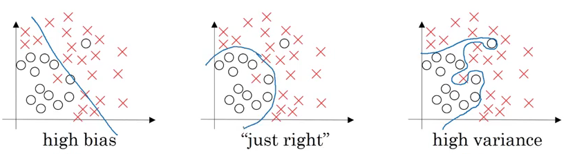
We want our model to be just right, which means having low bias and low variance. We can decide if the model should have high bias or high variance by checking the train set and dev set error. Generally, we can define it as:
- If the dev set error is much more than the train set error, the model is overfitting and has a high variance
- When both train and dev set errors are high, the model is underfitting and has a high bias
- If the train set error is high and the dev set error is even worse, the model has both high bias and high variance
- And when both the train and dev set errors are small, the model fits the data reasonably and has low bias and low variance
Basic Recipe for Machine Learning
I have a very simple method of dealing with certain problems I face in machine learning. Ask a set of questions and then figure out the answers one-by-one. It has proven to be extremely helpful for me in my journey and more often than not has led to improvements in the model’s performance. These questions are listed below:
Question 1: Does the model have high bias?
Solution: We can figure out whether the model has high bias by looking at the training set error. High training error results in high bias. In such cases, we can try bigger networks, train models for a longer period of time, or try different neural network architectures.
Question 2: Does the model have high variance?
Solution : If the dev set error is high, we can say that the model has high variance. To reduce the variance, we can get more data, use regularization, or try different neural network architectures.
One of the most popular techniques to reduce variance is called regularization. Let’s look at this concept and how it applies to neural networks in part II.
Part II: Regularizing your Neural Network
We can reduce the variance by increasing the amount of data. But is that really a feasible option every time? Perhaps there is no other data available, and if there is, it might be too expensive for your project to source. This is quite a common problem. And that’s why the concept of regularization plays an important role in preventing overfitting.
Regularization
Let’s take the example of logistic regression. We try to minimize the loss function: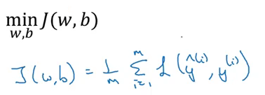
Now, if we add regularization to this cost function, it will look like: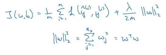 This is called L2 regularization. ƛ is the regularization parameter which we can tune while training the model. Now, let’s see how to use regularization for a neural network. The cost function for a neural network can be written as:
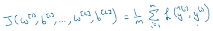
We can add a regularization term to this cost function (just like we did in our logistic regression equation):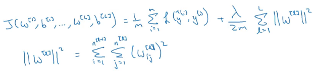
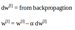
Finally, let’s see how regularization works for a gradient descent algorithm:
- Update equation without regularization is given by:
- Regularized form of these update equations will be:
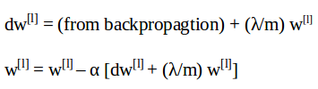
As you can surmise from the above equations, the reduction in weights will be more in case of regularization (since we are adding a higher quantity from the weights). This is the reason L2 regularization is also known as weight decay.
You must be wondering at this point how in the world does regularization prevent overfitting in the model? Let’s try to understand it in the next section.
How does regularization reduce overfitting?
The primary reason overfitting happens is because the model learns even the tiniest details present in the data. So after learning all the possible patterns it can find, the model tends to perform extremely well on the training set but fails to produce good results on the dev and test sets. It falls apart when faced with previously unseen data.
One way to prevent overfitting is to reduce the complexity of the model. This is exactly what regularization does! If we set the regularization parameter (ƛ) to a large value, the decay in the weights during gradient descent update will be more. Hence, the weights of most of the hidden units will be close to zero.
Since the weights are negligible, the model will not learn much from these units.This will end up making the network simpler and thus reduce overfitting:
Let’s understand this concept through one more example. Suppose we use the tanh activation function: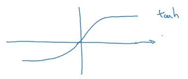
Now, if we set ƛ to a large value, the weight of the units w[l] will be less. To calculate the z[l] value, we will use the following formula:
z[l] = w[l] a[l-1] + b[l]
Hence, the z-value will be less. If we use the tanh activation function, these low values of z[l] will lie near the origin:
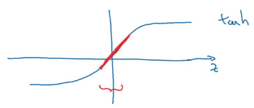
Here we are using only the linear region of the tanh function. This will make every layer in the network roughly linear, i.e., we will get linear boundaries that separate the data, thus preventing overfitting.
Dropout Regularization
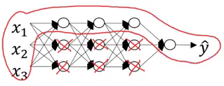
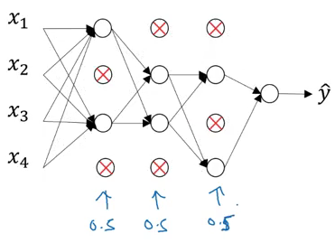
There is one more technique we can use to perform regularization. Consider you are building a neural network as shown below: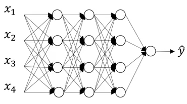
This neural network is overfitting on the training data. Suppose we add a dropout of 0.5 to all these images. The model will randomly remove 50% of the units from each layer and we finally end up with a much simpler network: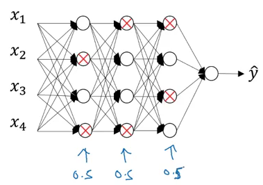
This has proven to be a very effective regularization technique. How can we implement it ourselves? Let’s check it out!
We will be working on this very example where we have three hidden layers. For now, we will consider the third layer, l=3. The dropout vector d for the third hidden layer can be written as:
d3 = np.random.rand(a3.shape[0], a3.shape[1]) < keep_prob
Here, keep_prob is the probability of keeping a unit. Now, we will calculate the activations for the selected units:
a3 = np.multiply(a3,d3)
This a3 value will be reduced by a factor of (1-keep_probs). So to get the expected value of a3, we divide the value:
a3 /= keep_dims
Let’s understand the concept of dropout using an example:
Number of units in the layer = 50

keep_prob = 0.8
So, 20% of the total units (i.e. 10) will be randomly shut off.
Different sets of hidden layers are dropped randomly in each training iteration. Note that dropout is only done at the time of training the model (not during the test phase). The reason for doing this is because:
- We don’t want our outputs to be random
- Dropout adds noise to the predictions
Other Regularization Methods
Apart from L2 regularization and dropout, there are a few other techniques that can be used to reduce overfitting.
- Data Augmentation: Suppose we are building an image classification model and are lacking the requisite data due to various reasons. In such cases, we can use data augmentation, i.e., applying some changes such as flipping the image, taking random crops of the image, randomly rotating images, etc. These can potentially help us get more training data and hence reduce overfitting.
- Early Stopping: To understand this, consider the below example:
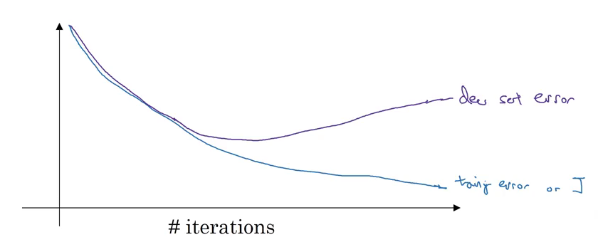
Here, the training error is continuously decreasing with respect to time. On the other hand, the dev set error is decreasing initially before increasing after a few iterations. We can stop the training at the point where the dev set error starts to increase. This, in a nutshell, is called early stopping.
And that is a wrap as far as regularization techniques are concerned!
Part III: Setting up your Optimization Problem
In this module, we will discuss the different techniques that can be used to speed up the training process.
Normalizing Inputs
Suppose we have 2 input features and their scatter plot looks like this: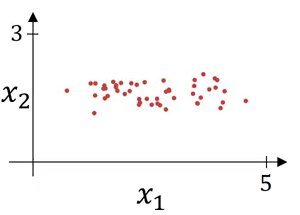
This is how we can represent the input as a vector: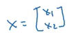
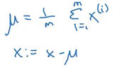
We’ll follow the below steps to normalize the input:
- Subtract the mean from the input features:
This will change the scatter plot from what is shown above to (notice that the variables have much higher variance in this graph):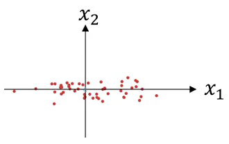
- Next, we normalize the variance:
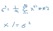
We divide the features with the variance. This will make the input look like: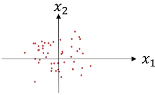
A key point to note is that we use the same mean and variance to normalize the test set as well. We should do this because we want the same transformation to happen on both the train and test data.
But why does normalizing the data make the algorithm faster?
In the case of unnormalized data, the scale of features will vary, and hence there will be a variation in the parameters learnt for each feature. This will make the cost function asymmetric: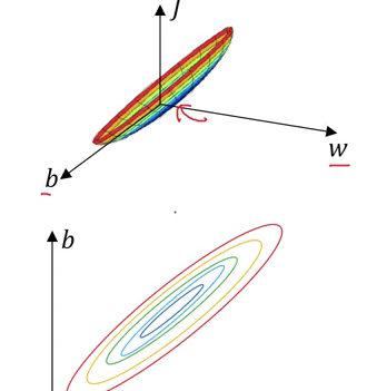
Whereas, in the case of normalized data, the scale will be the same and the cost function will also be symmetric: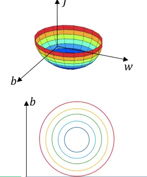
Normalizing the inputs makes the cost function symmetric. This makes it is easier for the gradient descent algorithm to find the global minima more quickly. And this, in turn, makes the algorithm run much faster.
Vanishing / Exploding gradients
While training deep neural networks, sometimes the derivatives (slopes) can become either very big or very small. It can make the training phase quite difficult. This is the problem of vanishing / exploding gradients. Suppose we are using a neural network with ‘l’ layers with two input features and we initialized the large weights: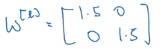
The final output at the lth layer will be (consider we are using a linear activation function):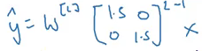
For deeper networks, L will be large, making the gradients very large and the learning process slow. Similarly, using small weights will make the gradients very small, and as a result, learning will be slow. We must deal with this problem in order to reduce the training time. So how should the weights be initialized?
Weight Initialization for Deep Networks
One potential solution to this problem can be random initialization. Consider a single neuron as shown below: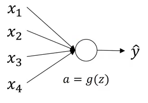
For this example, we can initialize the weights as: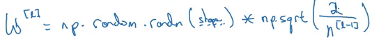
The primary reason behind initializing the weights randomly is to break symmetry. We want to make sure that different hidden units learn different patterns. There is one more technique that can help ensure that our implementations are correct and will run quickly.
Gradient Checking
Gradient checking is used to find bugs (if any) in the implementation of backpropagation. Consider the following graph: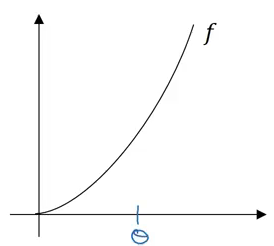
The derivative of the function w.r.to Θ can be best expressed as: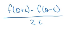
Where ε is the small step which we take towards the left and right of Θ. Make sure that the derivative calculated above is nearly equal to the actual derivative of the function. Below are the steps we follow for gradient checking:
- Take W[1], b[1],…., w[L], b[L] and reshape it into a big vector Θ:
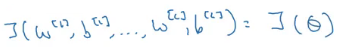
- We also calculate dW[1], db[1],…, dw[L], db[L] and reshape it into a big vector dΘ
- Finally, we check whether dΘ is the gradient of J(Θ)
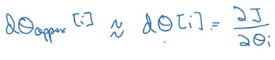
For each i, we calculate:
We use Euclidean distance (ε) to measure whether both these terms are equal: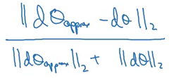
We want this value to be as small as possible. So, if ε is 10-7, we say it is a great approximation, If ε is 10-5, it is acceptable, and if ε is in the range 10-3, we have to change the approximations and recalculate the weights.
And that’s a wrap for module 1!
Module 2: Optimization Algorithms
The objectives behind this module are:
- To learn different optimization methods such as (Stochastic) Gradient Descent, Momentum, RMSProp and Adam
- Using random mini batches to accelerate the convergence and improve the optimization
- To know the benefits of learning rate decay and apply it to your optimization
Mini-Batch Gradient Descent
We saw in course 1 how vectorization can help us to effectively work with ‘m’ training examples. We can get rid of explicit for loops and make the training phase faster. So, we take the training examples as: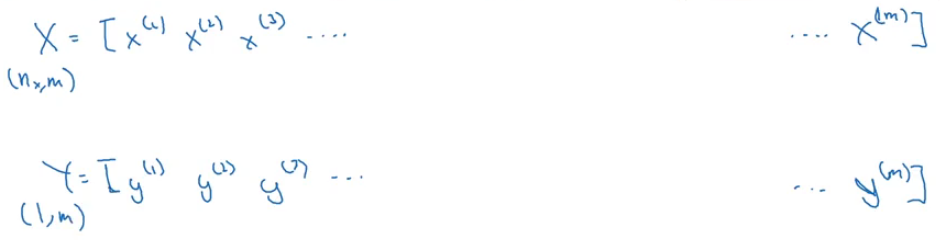
Where X is the vectorized input and Y is their corresponding outputs. But what will happen if we have a large training set, say m = 5,000,000? If we process through all of these training examples in every training iteration, the gradient descent update will take a lot of time. Instead, we can use a mini batch of the training examples and update the weights based on them.
Suppose we make a mini-batch containing 1000 examples each. This means we have 5000 batches and the training set will look like this: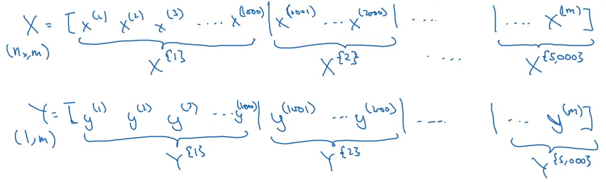
Here, X{t}, Y{t} represents the tth mini-batch input and output. Now, let’s look at how to implement a mini-batch gradient descent:
for t = 1:No_of_batches                         # this is called an epoch
    A[L], Z[L] = forward_prop(X{t}, Y{t})
    cost = compute_cost(A[L], Y{t})
    grads = backward_prop(A[L], caches)
    update_parameters(grads)
This is equivalent to 1 epoch (1 epoch = single pass through the training set). Note that the cost function for mini batch is given as:![]()
Where 1000 is the number of mini batches we saw in our above example. Let’s dive deeper and understand mini-batch gradient descent in detail.
Understanding Mini-Batch Gradient Descent
In batch gradient descent, our cost function should decrease on every single iteration: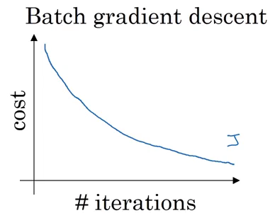
In the case of mini-batch gradient descent, we only use a specified set of training examples. As a result, the cost function can decrease for some iterations: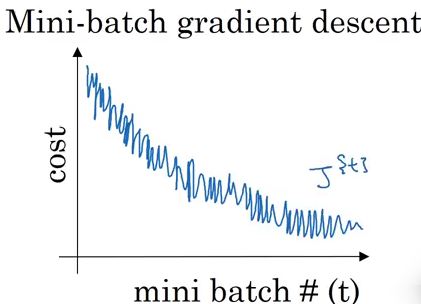
How can we choose a mini-batch size? Let’s see various cases:
- If the mini-batch size = m:
It is a batch gradient descent where all the training examples are used in each iteration. It takes too much time per iteration. - If the mini-batch size = 1:
It is called stochastic gradient descent, where each training example is its own mini-batch. Since in every iteration we are taking just a single example, it can become extremely noisy and takes much more time to reach the global minima. - If the mini-batch size is between 1 to m:
It is mini-batch gradient descent. The size of the mini-batch should not be too large or too small.
Below are a few general guidelines to keep in mind while deciding the mini-batch size:
- If the training set is small, we can choose a mini-batch size of m<2000
- For a larger training set, typical mini-batch sizes are: 64, 128, 256, 512
- Make sure that the mini-batch size fits your CPU/GPU memory
Exponentially weighted averages
Below is a sample of hypothetical temperature data collected for an entire year:
Θ1 = 40 F
Θ2 = 49 F
Θ3 = 45 F
.
.
Θ180 = 60 F
Θ181 = 56 F
.
.
The below plot neatly summarizes this temperature data for us: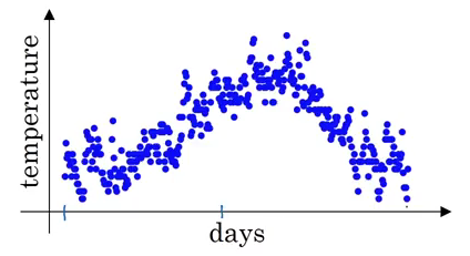
Exponentially weighted average, or exponentially weighted moving average, computes the trends. We will first initialize a term as 0:
V0 = 0
Now, all the further terms will be calculated as the weighted sum of V0 and the temperature of that day:
V1 = 0.9 * V0 + 0.1 * Θ1
V2 = 0.9 * V1 + 0.1 * Θ2
And so on. A more generalized form of exponentially weighted average can be written as:
Vt = β * V(t-1) + (1 – β) * Θt
Using this equation for trend, the data will be generalised as: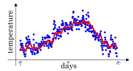
The β value in this example is 0.9, which means Vt is an approximation of average over 1/(1-β) days, i.e., 1/(1-0.9) = 10 days temperature. Increasing the value of β will result in approximating over more days, i.e., taking the average temperature of more days. If the β value is small, i.e., we use only 1 day’s data for approximation, the predictions become much more noisy: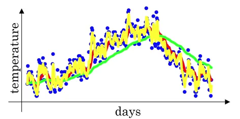
Here, the green line is the approximation when β = 0.98 (using 50 days) and the yellow line is when β = 0.5 (using 2 days). It can be seen that using small β results in noisy predictions.
The equation of exponentially weighted averages is given by:
Vt = β * V(t-1) + (1 – β) * Θt
Let’s look at how we can implement this:
Initialize VΘ = 0
Repeat
{
get next Θt
VΘ = β * VΘ + (1 - β) * Θt
}
This step takes a lot less memory as we are overwriting the previous values. Hence, it is a computational, as well as memory efficient, process.
Bias Correction in Exponentially Weighted Averages
We initialize V0 = 0, so while calculating the V1 value it will only be equal to (1 – β) * Θ1. It will not generalize well to the actual values. We need to use bias correction to overcome this challenge.
Instead of using the previous equation, i.e.,
Vt = β * V(t-1) + (1 – β) * Θt
we include a bias correction term:
Vt = [β * V(t-1) + (1 – β) * Θt] / (1 – βt)
When t is small, βt will be large, resulting in a smaller value of (1-βt). This will make the Vt value larger ensuring that our predictions are accurate.
Gradient Descent with Momentum
The underlying idea of gradient descent with momentum is to calculate the exponential weighted average of gradients and use them to update weights. Suppose we have a cost function whose contours look like this:
The red dot is the global minima, and we want to reach that point. Using gradient descent, the updates will look like: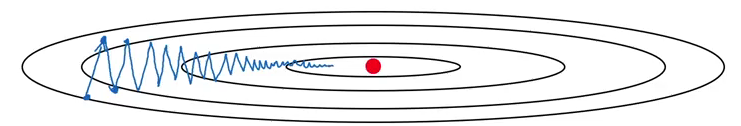
One more way could be to use a larger learning rate. But that could result in large upgrade steps, and we might not reach global minima. Additionally, too small a learning rate makes the gradient descent slower. We want a slower learning in the vertical direction and a faster learning in the horizontal direction which will help us to reach the global minima much faster.
Let’s see how we can achieve it using momentum:
On iteration t:
Compute dW, dB on current mini-batch using momentum
VdW = β * VdW + (1 - β) * dW
Vdb = β * Vdb + (1 - β) * db
Update weights
W = W - α * VdW
b = b - α * Vdb
Here, we have two hyperparameters, i.e., α and β. The role of dW and db in the above equation is to provide momentum, VdW and Vdb provides velocity, and β acts as friction and prevents speeding over the limit. Consider a ball rolling down – VdW and Vdb provide velocity to that ball and make it move faster. We do not want our ball to speed up so much that it misses the global minima, and hence β acts as friction.
Let me introduce you to a few more optimization algorithms.
RMSprop
Consider the example of a simple gradient descent:
Suppose we have two parameters w and b as shown below: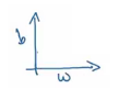
Look at the contour shown above and the parameters graph. We want to slow down the learning in b direction, i.e., the vertical direction, and speed up the learning in w direction, i.e., the horizontal direction. The steps followed in RMSprop can be summarised as:
On iteration t:
Compute dW, dB on current mini-batch
SdW = β2 * SdW + (1 - β2) * dW2
Vdb = β2 * Sdb + (1 - β2) * db2

Update weights
W = W - α * (dW/SdW)
b = b - α * (db/Sdb)
The slope in the vertical direction (db in our case) is steeper, resulting in a large value of Sdb. As we want slow learning in the vertical direction, dividing db with Sdbin update step will result in a smaller change in b. Hence, learning in the vertical direction will be less. Similarly, a small value of SdW will result in faster learning in the horizontal direction, thus making the algorithm faster.
Adam optimization algorithm
Adam is essentially a combination of momentum and RMSprop. Let’s see how we can implement it:
VdW = 0, SdW = 0, Vdb = 0, Sdb = 0
On iteration t:
Compute dW, dB on current mini-batch using momentum and RMSprop
VdW = β1 * VdW + (1 - β1) * dW
Vdb = β1 * Vdb + (1 - β1) * db

SdW = β2 * SdW + (1 - β2) * dW2
Sdb = β2 * Sdb + (1 - β2) * db2

Apply bias correction
VdWcorrected = VdW / (1 - β1t)
Vdbcorrected = Vdb / (1 - β1t)

SdWcorrected = SdW / (1 - β2t)
Sdbcorrected = Sdb / (1 - β2t)

Update weights
W = W - α * (VdWcorrected / SdWcorrected + ε)
b = b - α * (Vdbcorrected / Sdbcorrected + ε)
There are a range of hyperparameters used in Adam and some of the common ones are:
- Learning rate α: needs to be tuned
- Momentum term β1: common choice is 0.9
- RMSprop term β2: common choice is 0.999
- ε: 10-8
Adam helps to train a neural network model much more quickly than the techniques we have seen earlier.
Learning Rate Decay
If we slowly reduce the learning rate over time, we might speed up the learning process. This process is called learning rate decay.
Initially, when the learning rate is not very small, training will be faster. If we slowly reduce the learning rate, there is a higher chance of coming close to the global minima.
Learning rate decay can be given as:
α = [1 / (1 + decay_rate * epoch_number)] * α0
Let’s understand it with an example. Consider:
- α0 = 0.2
- decay_rate = 1
| epoch_number | α |
| 1 | [1/(1+1)]*0.2 = 0.1 |
| 2 | [1/(1+2)]*0.2 = 0.067 |
| 3 | 0.05 |
| 4 | 0.04 |
This is how, after each epoch, there is a decay in the learning rate which helps us reach the global minima much more quickly. There are a few more learning rate decay methods:
- Exponential decay: α = (0.95)epoch_number * α0
- α = k / epochnumber1/2 * α0
- α = k / t1/2 * α0
Here, t is the mini-batch number.
This was all about optimization algorithms and module 2! Take a deep breath, we are about to enter the final module of this article.
Module 3: Hyperparameter tuning, Batch Normalization and Programming Frameworks
The primary objectives of module 3 are:
- To master the process of hyperparameter tuning
- To familiarize yourself with the concept of Batch Normalization
Much like the first module, this is further divided into three sections:
- Part I: Hyperparameter tuning
- Part II: Batch Normalization
- Part III: Multi-class classification
Part I: Hyperparameter tuning
Tuning process
Hyperparameters. We see this term popularly being bandied about in data science competitions and hackathons. But how important is it in the overall scheme of things?
Tuning these hyperparameters effectively can lead to a massive improvement in your position on the leaderboard. Following are a few common hyperparameters we frequently work with in a deep neural network:
- Learning rate – α
- Momentum – β
- Adam’s hyperparameter – β1, β2, ε
- Number of hidden layers
- Number of hidden units for different layers
- Learning rate decay
- Mini-batch size
Learning rate usually proves to be the most important among the above. This is followed by the number of hidden units, momentum, mini-batch size, the number of hidden layers, and then the learning rate decay.
Now, suppose we have two hyperparameters. We sample the points in a grid and then systematically explore these values. Consider a five-by-five grid: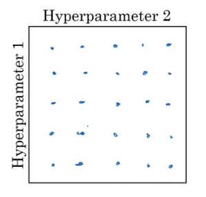
We check all 25 values and pick whichever hyperparameter works best. Instead of using these grids, we can try random values as well. Why? Because we do not know which hyperparameter value might turn out to be important, and in a grid we only define particular values.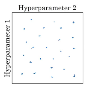
The major takeaway from this sub-section is to use random sampling and adequate search.
Using an Appropriate Scale to Pick Hyperparameters
To understand this, consider the number of hidden units hyperparameter. The range we are interested in is from 50 to 100. We can use a grid which contains values between 50 and 100 and use that to find the best value: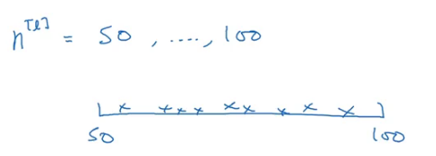
Now consider the learning rate with a range between 0.0001 and 1. If we draw a number line with these extreme values and sample the values uniformly at random, around 90% of the values will fall between 0.1 to 1. In other words, we are using 90% resources to search between 0.1 to 1, and only 10% to search between 0.0001 to 0.1. This does not look correct! Instead, we can use a log scale to choose the values: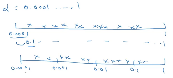
Next, we will learn a technique which makes our neural network much more robust to the choice of hyperparameters and also makes the training phase even more faster.
Part II: Batch Normalization
Normalizing Activations in a Network
Let’s recall how a logistic regression looks like: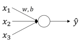
We have seen how normalizing the input in this case can speed up the learning process. In case of deep neural networks, we have a lot of hidden layers and this results in a lot of activations: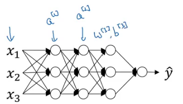
Wouldn’t it be great if we can normalize the mean and variance of these activations (a[2]) in order to make the training of w[3], b[3] more effective? This is how batch normalization works. We normalize the activations of the hidden layer(s) so that the weights of the next layer can be updated faster. Technically, we normalize the values of z[2] and then use an activation function of the normalized values. Here is how we can implement batch normalization:
Given some intermediate values in NN Z(1),….,Z(m):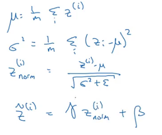
Here, Ɣ and β are learnable parameters.
Fitting Batch Norm into a Neural Network
Consider the neural network shown below: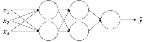
Each unit of the neural network computes two things. It first computes Z, and then applies the activation function on it to compute A. If we apply batch norm at each layer, the computation will look like: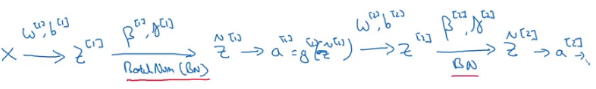
After calculating the Z-value, we apply batch norm and then the activation function on that. Parameters in this case are: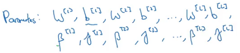
Finally, let’s see how we can apply gradient descent using batch norm:
For t=1, ….., number of batches:
    Compute forward propagation on X{t}
    In each hidden layer, use batch normalization
    Use backpropagation to compute dW[l], db[l], dβ[l] and dƔ[l]
    Update the parameters:
    W[l] = W[l] - α*dW[l]
    β[l] = β[l] - α*dβ[l]
Note that this also works with momentum, RMSprop and Adam.
How does Batch Norm work?
In the case of logistic regression, we now know how normalizing the inputs helps to speed up the learning. Batch norm works in much the same way. Let’s take one more use case to understand it better. Consider the training set for a binary classification problem: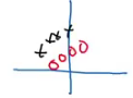
But when we try to generalize it to a dataset having different distribution, say: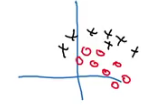
The decision boundary in both the cases might be same: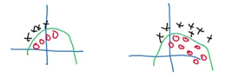
But the model would not be able to discover this green decision boundary. So, as the distribution of the input changes, we might have to train the model again. Consider a deep neural network: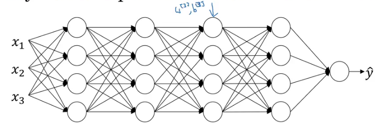
And let’s only consider the learning of layer 3. It will have activations from layer two as its input: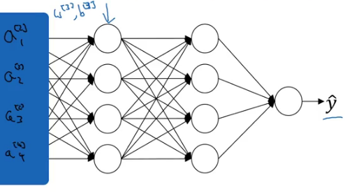
The aim of the third hidden layer is to take these activations and map them with the output. These activations change every time as the parameters of the previous layers change. Hence, we see a lot of shift in the activation values. Batch norm reduces the amount that the distribution of these hidden unit values shift around.
Additionally, it turns out that batch norm has a regularization effect as well:
- Each mini-batch is normalized using the mean / variance computed just on that mini batch
- This adds some noise to the values of z[l] within that mini batch, which is similar to the effect of dropout
- Hence this has a slight effect of regularization as well
One thing to note is that while making predictions, there is a slight difference in the way we use batch normalization.
Batch Norm at Test Time
We need to process the examples one at a time when making predictions on the test data. In the training period, the steps of batch norm can be written as: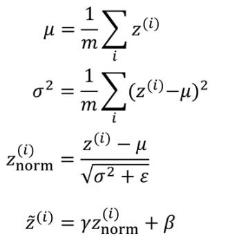
We first calculate the mean and variance of that mini-batch, and use that to normalize the z-value. We will be using the entire mini-batch to calculate the mean and standard deviation. We process each image separately, so taking the mean and standard deviation of a single image does not make sense.
We use exponentially weighted average to calculate the mean and variance across different mini-batches. Finally, we use these values to scale the test data.
Part III: Multi-Class Classification
Softmax Regression
Binary classification means dealing with two classes. But when we have more than two classes in a problem, that is called multi-class classification. Suppose we have to recognize cats, dogs and tigers in a set of images. How many types of classes are there? 4 – cat, dog, tiger and none of them. If you said three there then think again!
For solving such problems, we use softmax regression. At the output layer, instead of having a single unit, we have units equal to the total number of classes (4 in our case). Each unit tells us the probability of the image falling in different classes. Since it tells the probability, the sum of values from each unit is always equal to 1.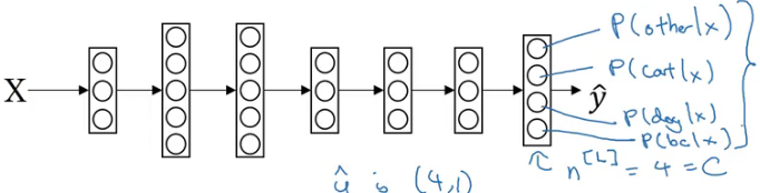
This is how a neural network for a multi-class classification looks like. So, for layer L, the output will be:
Z[L] = W[L]*a[L-1] + b[L]
The activation function will be: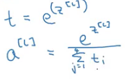
Let’s understand this with an example. Consider the output from the last hidden layer: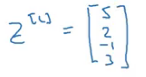
We then calculate t using the formula given above: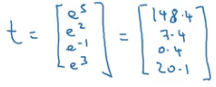
Finally, we calculate the activations: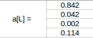
This is how we can solve a multi-class classification problem using the softmax activation function. And that brings us to the end of course 2!
End Notes
Congratulations! We have completed the second course of the deep learning specialization. It was quite an intense exercise writing this article and it really helped solidify my own concepts in the process. To summarize what we covered here:
- We now know how to improve the performance of our neural network using various techniques
- We first saw how deciding the train/dev/test split helps us in deciding which model will perform best
- Then we saw how regularization helps us to deal with overfitting
- We covered how to setup an optimization problem
- We also looked at various optimization algorithms like momentum, RMSprop, Adam which help us reach the global minima of a cost function faster and hence reduce the learning time
- We learned how to tune various hyperparameters in a neural network model and how scaling can help us achieve that
- Finally, we covered the Batch normalization technique, which we can use to further speed up the training time
If you have any feedback on this article or have any doubts/questions, kindly share them in the comments section below.
My research interests lies in the field of Machine Learning and Deep Learning. Possess an enthusiasm for learning new skills and technologies.


I am deeply challenged as a researcher in concrete materials. Can you further improve my knowledge on the applicability of this to my areas of research?
Thanks for your efforts to compile this! There are many things which I couldn't understand well by watching the videos but they were clear in your notes. Looking forward for the next 3 :)
Glad that you liked it Vishnu!!
Such a complete note. Thanks a ton, pulkit. Kindly, let us know when we can expect the part-3 notes?
Hi Arun, The next part has been published.