Predicting Movie Genres using NLP – An Awesome Introduction to Multi-Label Classification

Introduction

I was intrigued going through this amazing article on building a multi-label image classification model last week. The data scientist in me started exploring possibilities of transforming this idea into a Natural Language Processing (NLP) problem.

That article showcases computer vision techniques to predict a movie’s genre. So I had to find a way to convert that problem statement into text-based data. Now, most NLP tutorials look at solving single-label classification challenges (when there’s only one label per observation).

But movies are not one-dimensional. One movie can span several genres. Now THAT is a challenge I love to embrace as a data scientist. I extracted a bunch of movie plot summaries and got down to work using this concept of multi-label classification. And the results, even using a simple model, are truly impressive.

In this article, we will take a very hands-on approach to understanding multi-label classification in NLP. I had a lot fun building the movie genre prediction model using NLP and I’m sure you will as well. Let’s dig in!

Table of Contents

1. Brief Introduction to Multi-Label Classification
2. Setting up our Multi-Label Classification Problem Statement
3. About the Dataset
4. Our Strategy to Build a Movie Genre Prediction Model
5. Implementation: Using Multi-Label Classification to Build a Movie Genre Prediction Model (in Python)

Brief Introduction to Multi-Label Classification

I’m as excited as you are to jump into the code and start building our genre classification model. Before we do that, however, let me introduce you to the concept of multi-label classification in NLP. It’s important to first understand the technique before diving into the implementation.

The underlying concept is apparent in the name – multi-label classification. Here, an instance/record can have multiple labels and the number of labels per instance is not fixed.

Let me explain this using a simple example. Take a look at the below tables, where ‘X’ represents the input variables and ‘y’ represents the target variables (which we are predicting):

• ‘y’ is a binary target variable in Table 1. Hence, there are only two labels – t1 and t2
• ‘y’ contains more than two labels in Table 2. But, notice how there is only one label for every input in both these tables
• You must have guessed why Table 3 stands out. We have multiple tags here, not just across the table, but for individual inputs as well

We cannot apply traditional classification algorithms directly on this kind of dataset. Why? Because these algorithms expect a single label for every input, when instead we have multiple labels. It’s an intriguing challenge and one that we will solve in this article.

You can get a more in-depth understanding of multi-label classification problems in the below article:

• Solving Multi-Label Classification Problems (using Case Studies)

Setting up our Multi-Label Classification Problem Statement

There are several ways of building a recommendation engine. When it comes to movie genres, you can slice and dice the data based on multiple variables. But here’s a simple approach – build a model that can automatically predict genre tags! I can already imagine the possibilities of adding such an option to a recommender. A win-win for everyone.

Our task is to build a model that can predict the genre of a movie using just the plot details (available in text form).

Take a look at the below snapshot from IMDb and pick out the different things on display:

There’s a LOT of information in such a tiny space:

• Movie title
• Movie rating in the top-right corner
• Total movie duration
• Release date
• And of course, the movie genres which I have highlighted in the magenta coloured bounding box

Genres tell us what to expect from the movie. And since these genres are clickable (at least on IMDb), they allow us to discover other similar movies of the same ilk. What seemed like a simple product feature suddenly has so many promising options. 🙂

About the Dataset

We will use the CMU Movie Summary Corpus open dataset for our project. You can download the dataset directly from this link.

This dataset contains multiple files, but we’ll focus on only two of them for now:

• movie.metadata.tsv: Metadata for 81,741 movies, extracted from the November 4, 2012 dump of Freebase. The movie genre tags are available in this file
• plot_summaries.txt: Plot summaries of 42,306 movies extracted from the November 2, 2012 dump of English-language Wikipedia. Each line contains the Wikipedia movie ID (which indexes into movie.metadata.tsv) followed by the plot summary

Our Strategy to Build a Movie Genre Prediction Model

We know that we can’t use supervised classification algorithms directly on a multi-label dataset. Therefore, we’ll first have to transform our target variable. Let’s see how to do this using a dummy dataset:

Here, X and y are the features and labels, respectively – it is a multi-label dataset. Now, we will use the Binary Relevance approach to transform our target variable, y. We will first take out the unique labels in our dataset:

Unique labels = [ t1, t2, t3, t4, t5 ]

There are 5 unique tags in the data. Next, we need to replace the current target variable with multiple target variables, each belonging to the unique labels of the dataset. Since there are 5 unique labels, there will be 5 new target variables with values 0 and 1 as shown below:

We have now covered the necessary ground to finally start solving this problem. In the next section, we will finally make an Automatic Movie Genre Prediction System using Python!

Implementation: Using Multi-Label Classification to Build a Movie Genre Prediction Model (in Python)

We have understood the problem statement and built a logical strategy to design our model. Let’s bring it all together and start coding!

Import the required libraries

We will start by importing the libraries necessary to our project:

Load Data

Let’s load the movie metadata file first. Use ‘\t’ as the separator as it is a tab separated file (.tsv):

Oh wait – there are no headers in this dataset. The first column is the unique movie id, the third column is the name of the movie, and the last column contains the movie genre(s). We will not use the rest of the columns in this analysis.

Let’s add column names to the aforementioned three variables:

# rename columns
meta.columns = ["movie_id",1,"movie_name",3,4,5,6,7,"genre"]

Now, we will load the movie plot dataset into memory. This data comes in a text file with each row consisting of a movie id and a plot of the movie. We will read it line-by-line:

Next, split the movie ids and the plots into two separate lists. We will use these lists to form a dataframe:

Let’s see what we have in the ‘movies’ dataframe:

movies.head()

Perfect! We have both the movie id and the corresponding movie plot.

Data Exploration and Pre-processing

Let’s add the movie names and their genres from the movie metadata file by merging the latter into the former based on the movie_id column:

Great! We have added both movie names and genres. However, the genres are in a dictionary notation. It will be easier to work with them if we can convert them into a Python list. We’ll do this using the first row:

movies['genre'][0]

Output:

'{"/m/07s9rl0": "Drama", "/m/03q4nz": "World cinema"}'

We can’t access the genres in this row by using just .values( ). Can you guess why? This is because this text is a string, not a dictionary. We will have to convert this string into a dictionary. We will take the help of the json library here:

type(json.loads(movies['genre'][0]))

Output:

dict

We can now easily access this row’s genres:

json.loads(movies['genre'][0]).values()

Output:

dict_values(['Drama', 'World cinema'])

This code helps us to extract all the genres from the movies data. Once done, add the extracted genres as lists back to the movies dataframe:

Some of the samples might not contain any genre tags. We should remove those samples as they won’t play a part in our model building process:

# remove samples with 0 genre tags
movies_new = movies[~(movies['genre_new'].str.len() == 0)]

movies_new.shape, movies.shape

Output:

((41793, 5), (42204, 5))

Only 411 samples had no genre tags. Let’s take a look at the dataframe once again:

movies.head()

Notice that the genres are now in a list format. Are you curious to find how many movie genres have been covered in this dataset? The below code answers this question:

# get all genre tags in a list
all_genres = sum(genres,[])
len(set(all_genres))

Output:

363

There are over 363 unique genre tags in our dataset. That is quite a big number. I can hardy recall 5-6 genres! Let’s find out what are these tags. We will use FreqDist( ) from the nltk library to create a dictionary of genres and their occurrence count across the dataset:

I personally feel visualizing the data is a much better method than simply putting out numbers. So, let’s plot the distribution of the movie genres:

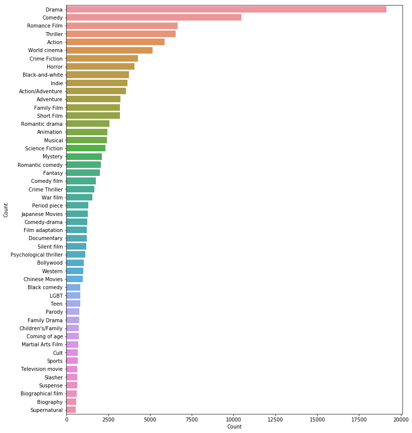
Next, we will clean our data a bit. I will use some very basic text cleaning steps (as that is not the focus area of this article):

Let’s apply the function on the movie plots by using the apply-lambda duo:

movies_new['clean_plot'] = movies_new['plot'].apply(lambda x: clean_text(x))

Feel free to check the new versus old movie plots. I have provided a few random samples below:

In the clean_plot column, all the text is in lowercase and there are also no punctuation marks. Our text cleaning has worked like a charm.

The function below will visualize the words and their frequency in a set of documents. Let’s use it to find out the most frequent words in the movie plots column:

Most of the terms in the above plot are stopwords. These stopwords carry far less meaning than other keywords in the text (they just add noise to the data). I’m going to go ahead and remove them from the plots’ text. You can download the list of stopwords from the nltk library:

nltk.download('stopwords')

Let’s remove the stopwords:

Check the most frequent terms sans the stopwords:

freq_words(movies_new['clean_plot'], 100)

Looks much better, doesn’t it? Far more interesting and meaningful words have now emerged, such as “police”, “family”, “money”, “city”, etc.

Converting Text to Features

I mentioned earlier that we will treat this multi-label classification problem as a Binary Relevance problem. Hence, we will now one hot encode the target variable, i.e., genre_new by using sklearn’s MultiLabelBinarizer( ). Since there are 363 unique genre tags, there are going to be 363 new target variables.

tfidf_vectorizer = TfidfVectorizer(max_df=0.8, max_features=10000)

Now we can create features for the train and the validation set:

# create TF-IDF features
xtrain_tfidf = tfidf_vectorizer.fit_transform(xtrain)
xval_tfidf = tfidf_vectorizer.transform(xval)

Build Your Movie Genre Prediction Model

We are all set for the model building part! This is what we’ve been waiting for.

Remember, we will have to build a model for every one-hot encoded target variable. Since we have 363 target variables, we will have to fit 363 different models with the same set of predictors (TF-IDF features).

As you can imagine, training 363 models can take a considerable amount of time on a modest system. Hence, I will build a Logistic Regression model as it is quick to train on limited computational power:

from sklearn.linear_model import LogisticRegression

# Binary Relevance
from sklearn.multiclass import OneVsRestClassifier

# Performance metric
from sklearn.metrics import f1_score

We will use sk-learn’s OneVsRestClassifier class to solve this problem as a Binary Relevance or one-vs-all problem:

lr = LogisticRegression()
clf = OneVsRestClassifier(lr)

Finally, fit the model on the train set:

# fit model on train data
clf.fit(xtrain_tfidf, ytrain)

Predict movie genres on the validation set:

# make predictions for validation set
y_pred = clf.predict(xval_tfidf)

Let’s check out a sample from these predictions:

y_pred[3]

It is a binary one-dimensional array of length 363. Basically, it is the one-hot encoded form of the unique genre tags. We will have to find a way to convert it into movie genre tags.

Luckily, sk-learn comes to our rescue once again. We will use the inverse_transform( ) function along with the MultiLabelBinarizer( ) object to convert the predicted arrays into movie genre tags:

multilabel_binarizer.inverse_transform(y_pred)[3]

Output:

('Action', 'Drama')

# evaluate performance
f1_score(yval, y_pred, average="micro")

Output:

0.31539641943734015

We get a decent F1 score of 0.315. These predictions were made based on a threshold value of 0.5, which means that the probabilities greater than or equal to 0.5 were converted to 1’s and the rest to 0’s.

Let’s try to change this threshold value and see if that improves our model’s score:

# predict probabilities
y_pred_prob = clf.predict_proba(xval_tfidf)

Now set a threshold value:

t = 0.3 # threshold value
y_pred_new = (y_pred_prob >= t).astype(int)

I have tried 0.3 as the threshold value. You should try other values as well. Let’s check the F1 score again on these new predictions.

# evaluate performance
f1_score(yval, y_pred_new, average="micro")

Output:

0.4378456703198025

That is quite a big boost in our model’s performance. A better approach to find the right threshold value would be to use a k-fold cross validation setup and try different values.

Create Inference Function

Wait – we are not done with the problem yet. We also have to take care of the new data or new movie plots that will come in the future, right? Our movie genre prediction system should be able to take a movie plot in raw form as input and generate its genre tag(s).

To achieve this, let’s build an inference function. It will take a movie plot text and follow the below steps:

• Clean the text
• Remove stopwords from the cleaned text
• Extract features from the text
• Make predictions
• Return the predicted movie genre tags

Let’s test this inference function on a few samples from our validation set:

Yay! We’ve built a very serviceable model. The model is not yet able to predict rare genre tags but that’s a challenge for another time (or you could take it up and let us know the approach you followed).

Where to go from here?

If you are looking for similar challenges, you’ll find the below links useful. I have solved a Stackoverflow Questions Tag Prediction problem using both machine learning and deep learning models in our course on Natural Language Processing.

The links to the course are below for your reference:

• Certified Course: Natural Language Processing (NLP) using Python
• Certified Program: NLP for Beginners
• The Ultimate AI & ML BlackBelt Program

End Notes

I would love to see different approaches and techniques from our community to achieve better results. Try to use different feature extraction methods, build different models, fine-tune those models, etc. There are so many things that you can try. Don’t stop yourself here – go on and experiment!

Feel free to discuss and comment in the comment section below. The full code is available here.

Prateek Joshi 19 Jul 2022

Data Scientist at Analytics Vidhya with multidisciplinary academic background. Experienced in machine learning, NLP, graphs & networks. Passionate about learning and applying data science to solve real world problems.