10 Powerful Applications of Linear Algebra in Data Science (with Multiple Resources)
Overview
- Linear algebra powers various and diverse data science algorithms and applications
- Here, we present 10 such applications where linear algebra will help you become a better data scientist
- We have categorized these applications into various fields – Basic Machine Learning, Dimensionality Reduction, Natural Language Processing, and Computer Vision
Introduction
If Data Science was Batman, Linear Algebra would be Robin. This faithful sidekick is often ignored. But in reality, it powers major areas of Data Science including the hot fields of Natural Language Processing and Computer Vision.
I have personally seen a LOT of data science enthusiasts skip this subject because they find the math too difficult to understand. When the programming languages for data science offer a plethora of packages for working with data, people don’t bother much with linear algebra.
That’s a mistake. Linear algebra is behind all the powerful machine learning algorithms we are so familiar with. It is a vital cog in a data scientists’ skillset. As we will soon see, you should consider linear algebra as a must-know subject in data science.

And trust me, Linear Algebra really is all-pervasive! It will open up possibilities of working and manipulating data you would not have imagined before.
In this article, I have explained in detail ten awesome applications of Linear Algebra in Data Science. I have broadly categorized the applications into four fields for your reference:
I have also provided resources for each application so you can deep dive further into the one(s) which grabs your attention.
Note: Before you read on, I recommend going through this superb article – Linear Algebra for Data Science. It’s not mandatory for understanding what we will cover here but it’s a valuable article for your budding skillset.
Table of Contents
- Why Study Linear Algebra?
- Linear Algebra in Machine Learning
- Loss functions
- Regularization
- Covariance Matrix
- Support Vector Machine Classification
- Linear Algebra in Dimensionality Reduction
- Principal Component Analysis (PCA)
- Singular Value Decomposition (SVD)
- Linear Algebra in Natural Language Processing
- Word Embeddings
- Latent Semantic Analysis
- Linear Algebra in Computer Vision
- Image Representation as Tensors
- Convolution and Image Processing
Why Study Linear Algebra?
I have come across this question way too many times. Why should you spend time learning Linear Algebra when you can simply import a package in Python and build your model? It’s a fair question. So, let me present my point of view regarding this.
I consider Linear Algebra as one of the foundational blocks of Data Science. You cannot build a skyscraper without a strong foundation, can you? Think of this scenario:
You want to reduce the dimensions of your data using Principal Component Analysis (PCA). How would you decide how many Principal Components to preserve if you did not know how it would affect your data? Clearly, you need to know the mechanics of the algorithm to make this decision.
With an understanding of Linear Algebra, you will be able to develop a better intuition for machine learning and deep learning algorithms and not treat them as black boxes. This would allow you to choose proper hyperparameters and develop a better model.
You would also be able to code algorithms from scratch and make your own variations to them as well. Isn’t this why we love data science in the first place? The ability to experiment and play around with our models? Consider linear algebra as the key to unlock a whole new world.
Linear Algebra in Machine Learning
The big question – where does linear algebra fit in machine learning? Let’s look at four applications you will all be quite familiar with.
1. Loss Functions
You must be quite familiar with how a model, say a Linear Regression model, fits a given data:
- You start with some arbitrary prediction function (a linear function for a Linear Regression Model)
- Use it on the independent features of the data to predict the output
- Calculate how far-off the predicted output is from the actual output
- Use these calculated values to optimize your prediction function using some strategy like Gradient Descent
But wait – how can you calculate how different your prediction is from the expected output? Loss Functions, of course.
A loss function is an application of the Vector Norm in Linear Algebra. The norm of a vector can simply be its magnitude. There are many types of vector norms. I will quickly explain two of them:
- L1 Norm: Also known as the Manhattan Distance or Taxicab Norm. The L1 Norm is the distance you would travel if you went from the origin to the vector if the only permitted directions are parallel to the axes of the space.
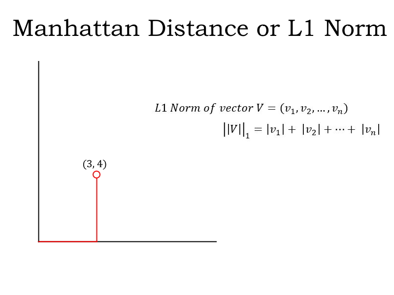 In this 2D space, you could reach the vector (3, 4) by traveling 3 units along the x-axis and then 4 units parallel to the y-axis (as shown). Or you could travel 4 units along the y-axis first and then 3 units parallel to the x-axis. In either case, you will travel a total of 7 units.
- L2 Norm: Also known as the Euclidean Distance. L2 Norm is the shortest distance of the vector from the origin as shown by the red path in the figure below:
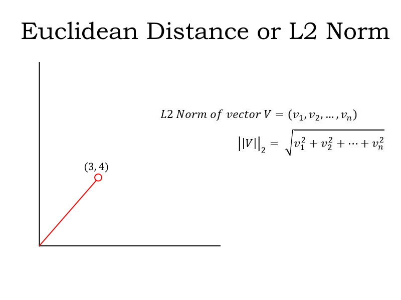 This distance is calculated using the Pythagoras Theorem (I can see the old math concepts flickering on in your mind!). It is the square root of (3^2 + 4^2), which is equal to 5.
But how is the norm used to find the difference between the predicted values and the expected values? Let’s say the predicted values are stored in a vector P and the expected values are stored in a vector E. Then P-E is the difference vector. And the norm of P-E is the total loss for the prediction.
2. Regularization
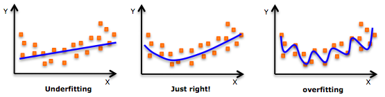
Regularization is a very important concept in data science. It’s a technique we use to prevent models from overfitting. Regularization is actually another application of the Norm.
A model is said to overfit when it fits the training data too well. Such a model does not perform well with new data because it has learned even the noise in the training data. It will not be able to generalize on data that it has not seen before. The below illustration sums up this idea really well:
Regularization penalizes overly complex models by adding the norm of the weight vector to the cost function. Since we want to minimize the cost function, we will need to minimize this norm. This causes unrequired components of the weight vector to reduce to zero and prevents the prediction function from being overly complex.
You can read the below article to learn about the complete mathematics behind regularization:
The L1 and L2 norms we discussed above are used in two types of regularization:
- L1 regularization used with Lasso Regression
- L2 regularization used with Ridge Regression
Refer to our complete tutorial on Ridge and Lasso Regression in Python to know more about these concepts.
3. Covariance Matrix
Bivariate analysis is an important step in data exploration. We want to study the relationship between pairs of variables. Covariance or Correlation are measures used to study relationships between two continuous variables.
Covariance indicates the direction of the linear relationship between the variables. A positive covariance indicates that an increase or decrease in one variable is accompanied by the same in another. A negative covariance indicates that an increase or decrease in one is accompanied by the opposite in the other.
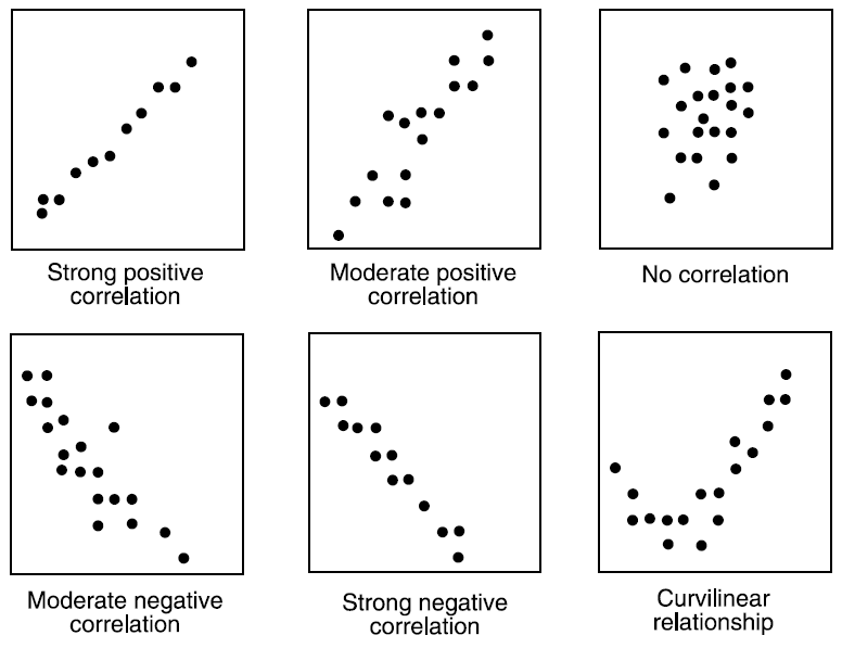
On the other hand, correlation is the standardized value of Covariance. A correlation value tells us both the strength and direction of the linear relationship and has the range from -1 to 1.
Now, you might be thinking that this is a concept of Statistics and not Linear Algebra. Well, remember I told you Linear Algebra is all-pervasive? Using the concepts of transpose and matrix multiplication in Linear Algebra, we have a pretty neat expression for the covariance matrix: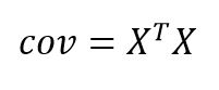
Here, X is the standardized data matrix containing all numerical features.
I encourage you to read our Complete Tutorial on Data Exploration to know more about the Covariance Matrix, Bivariate Analysis and the other steps involved in Exploratory Data Analysis.
4. Support Vector Machine Classification
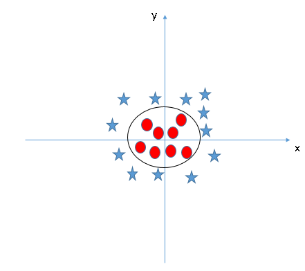
Ah yes, support vector machines. One of the most common classification algorithms that regularly produces impressive results. It is an application of the concept of Vector Spaces in Linear Algebra.
Support Vector Machine, or SVM, is a discriminative classifier that works by finding a decision surface. It is a supervised machine learning algorithm.
In this algorithm, we plot each data item as a point in an n-dimensional space (where n is the number of features you have) with the value of each feature being the value of a particular coordinate. Then, we perform classification by finding the hyperplane that differentiates the two classes very well i.e. with the maximum margin, which is C is this case.
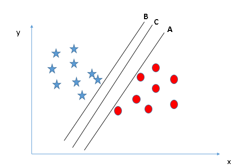
A hyperplane is a subspace whose dimensions are one less than its corresponding vector space, so it would be a straight line for a 2D vector space, a 2D plane for a 3D vector space and so on. Again Vector Norm is used to calculate the margin.
But what if the data is not linearly separable like the case below?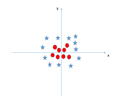
Our intuition says that the decision surface has to be a circle or an ellipse, right? But how do you find it? Here, the concept of Kernel Transformations comes into play. The idea of transformation from one space to another is very common in Linear Algebra.
Let’s introduce a variable z = x^2 + y^2. This is how the data looks if we plot it along the z and x-axes:
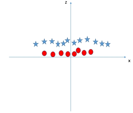
Now, this is clearly linearly separable by a line z = a, where a is some positive constant. On transforming back to the original space, we get x^2 + y^2 = a as the decision surface, which is a circle!
And the best part? We do not need to add additional features on our own. SVM has a technique called the kernel trick. Read this article on Support Vector Machines to learn about SVM, the kernel trick and how to implement it in Python.
Dimensionality Reduction
You will often work with datasets that have hundreds and even thousands of variables. That’s just how the industry functions. Is it practical to look at each variable and decide which one is more important?
That doesn’t really make sense. We need to bring down the number of variables to perform any sort of coherent analysis. This is what dimensionality reduction is. Now, let’s look at two commonly used dimensionality reduction methods here.
5. Principal Component Analysis (PCA)
Principal Component Analysis, or PCA, is an unsupervised dimensionality reduction technique. PCA finds the directions of maximum variance and projects the data along them to reduce the dimensions.
Without going into the math, these directions are the eigenvectors of the covariance matrix of the data.
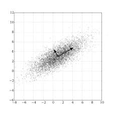
Eigenvectors for a square matrix are special non-zero vectors whose direction does not change even after applying linear transformation (which means multiplying) with the matrix. They are shown as the red-colored vectors in the figure below:

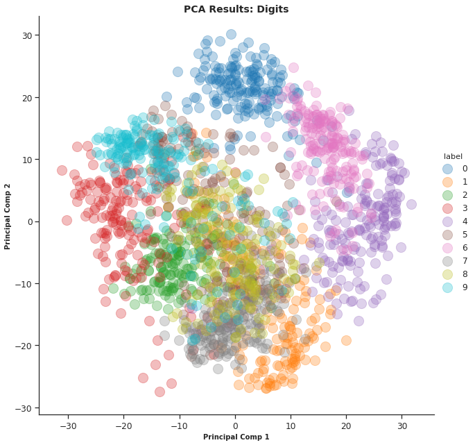
You can easily implement PCA in Python using the PCA class in the scikit-learn package:
I applied PCA on the Digits dataset from sklearn – a collection of 8×8 images of handwritten digits. The plot I obtained is rather impressive. The digits appear nicely clustered:
Head on to our Comprehensive Guide to 12 Dimensionality Reduction techniques with code in Python for a deeper insight into PCA and 11 other Dimensionality Reduction techniques. It is honestly one of the best articles on this topic you will find anywhere.
6. Singular Value Decomposition
In my opinion, Singular Value Decomposition (SVD) is underrated and not discussed enough. It is an amazing technique of matrix decomposition with diverse applications. I will try and cover a few of them in a future article.
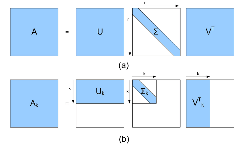
For now, let us talk about SVD in Dimensionality Reduction. Specifically, this is known as Truncated SVD.
- We start with the large m x n numerical data matrix A, where m is the number of rows and n is the number of features
- Decompose it into 3 matrices as shown here:
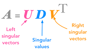
Source: hadrienj.github.io
- Choose k singular values based on the diagonal matrix and truncate (trim) the 3 matrices accordingly:

Source: researchgate.net
- Finally, multiply the truncated matrices to obtain the transformed matrix A_k. It has the dimensions m x k. So, it has k features with k < n
Here is the code to implement truncated SVD in Python (it’s quite similar to PCA):
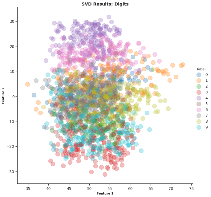
On applying truncated SVD to the Digits data, I got the below plot. You’ll notice that it’s not as well clustered as we obtained after PCA:
Natural Language Processing (NLP)
Natural Language Processing (NLP) is the hottest field in data science right now. This is primarily down to major breakthroughs in the last 18 months. If you were still undecided on which branch to opt for – you should strongly consider NLP.
So let’s see a couple of interesting applications of linear algebra in NLP. This should help swing your decision!
7. Word Embeddings
Machine learning algorithms cannot work with raw textual data. We need to convert the text into some numerical and statistical features to create model inputs. There are many ways for engineering features from text data, such as:
- Meta attributes of a text, like word count, special character count, etc.
- NLP attributes of text using Parts-of-Speech tags and Grammar Relations like the number of proper nouns
- Word Vector Notations or Word Embeddings
Word Embeddings is a way of representing words as low dimensional vectors of numbers while preserving their context in the document. These representations are obtained by training different neural networks on a large amount of text which is called a corpus. They also help in analyzing syntactic similarity among words:
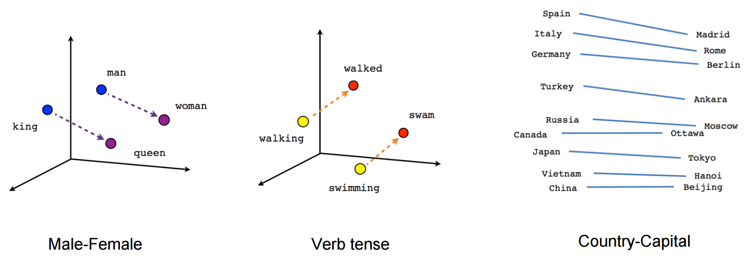
Word2Vec and GloVe are two popular models to create Word Embeddings.
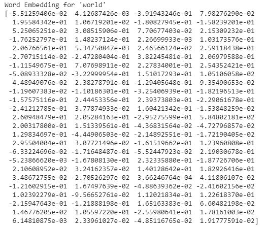
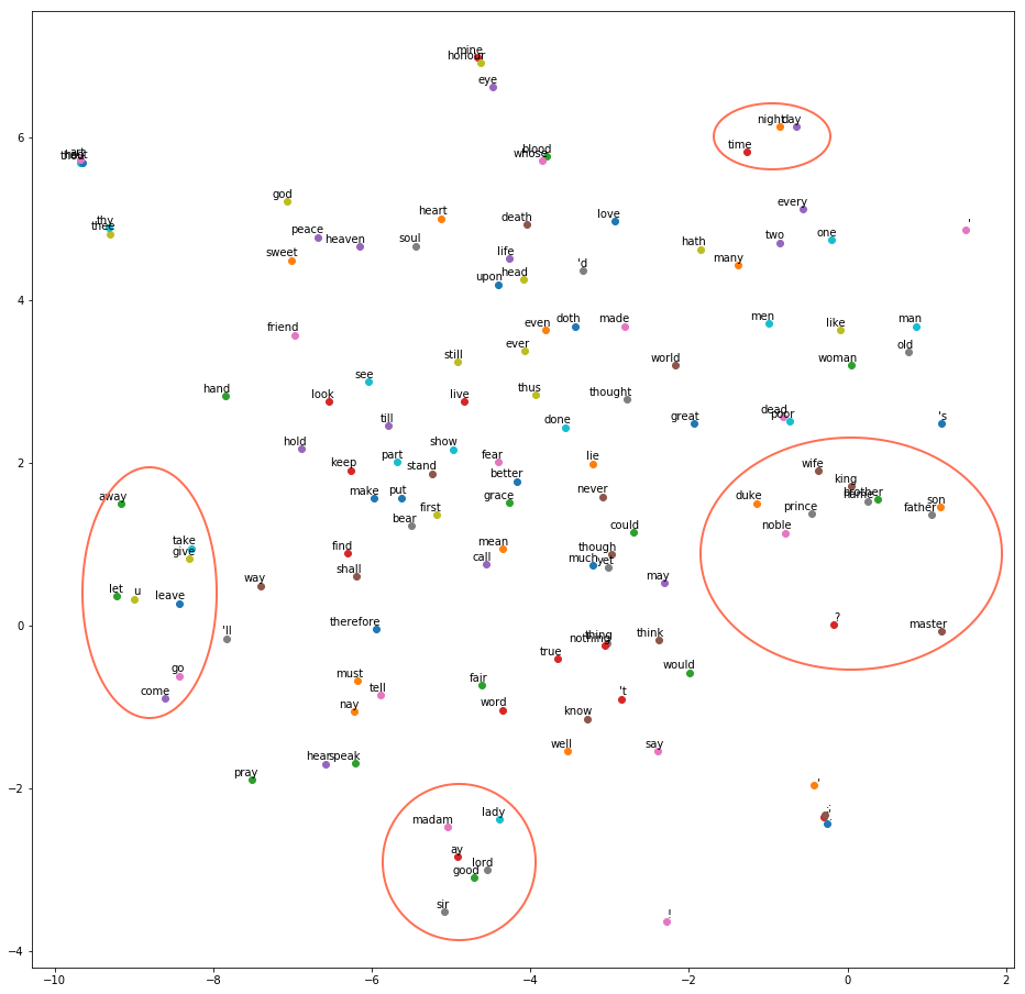
I trained my model on the Shakespeare corpus after some light preprocessing using Word2Vec and obtained the word embedding for the word ‘world’:
Pretty cool! But what’s even more awesome is the below plot I obtained for the vocabulary. Observe that syntactically similar words are closer together. I have highlighted a few such clusters of words. The results are not perfect but they are still quite amazing:
There are several other methods to obtain Word Embeddings. Read our article for An Intuitive Understanding of Word Embeddings: From Count Vectors to Word2Vec.
8. Latent Semantic Analysis (LSA)
What is your first thought when you hear this group of words – “prince, royal, king, noble”? These very different words are almost synonymous.
Now, consider the following sentences:
- The pitcher of the Home team seemed out of form
- There is a pitcher of juice on the table for you to enjoy
The word ‘pitcher’ has different meanings based on the other words in the two sentences. It means a baseball player in the first sentence and a jug of juice in the second.
Both these sets of words are easy for us humans to interpret with years of experience with the language. But what about machines? Here, the NLP concept of Topic Modeling comes into play:
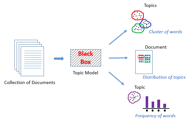
Topic Modeling is an unsupervised technique to find topics across various text documents. These topics are nothing but clusters of related words. Each document can have multiple topics. The topic model outputs the various topics, their distributions in each document, and the frequency of different words it contains.
Latent Semantic Analysis (LSA), or Latent Semantic Indexing, is one of the techniques of Topic Modeling. It is another application of Singular Value Decomposition.
Latent means ‘hidden’. True to its name, LSA attempts to capture the hidden themes or topics from the documents by leveraging the context around the words.
I will describe the steps in LSA in short so make sure you check out this Simple Introduction to Topic Modeling using Latent Semantic Analysis with code in Python for a proper and in-depth understanding.
- First, generate the Document-Term matrix for your data
- Use SVD to decompose the matrix into 3 matrices:
- Document-Topic matrix
- Topic Importance Diagonal Matrix
- Topic-term matrix
- Truncate the matrices based on the importance of topics
For a hands-on experience with Natural Language Processing, you can check out our course on NLP using Python. The course is beginner-friendly and you get to build 5 real-life projects!
Computer Vision
Another field of deep learning that is creating waves – Computer Vision. If you’re looking to expand your skillset beyond tabular data (and you should), then learn how to work with images.
This will broaden your current understanding of machine learning and also help you crack interviews quickly.
9. Image Representation as Tensors
How do you account for the ‘vision’ in Computer Vision? Obviously, a computer does not process images as humans do. Like I mentioned earlier, machine learning algorithms need numerical features to work with.
A digital image is made up of small indivisible units called pixels. Consider the figure below:
![]()
This grayscale image of the digit zero is made of 8 x 8 = 64 pixels. Each pixel has a value in the range 0 to 255. A value of 0 represents a black pixel and 255 represents a white pixel.
Conveniently, an m x n grayscale image can be represented as a 2D matrix with m rows and n columns with the cells containing the respective pixel values:
![]()
But what about a colored image? A colored image is generally stored in the RGB system. Each image can be thought of as being represented by three 2D matrices, one for each R, G and B channel. A pixel value of 0 in the R channel represents zero intensity of the Red color and of 255 represents the full intensity of the Red color.
Each pixel value is then a combination of the corresponding values in the three channels:


In reality, instead of using 3 matrices to represent an image, a tensor is used. A tensor is a generalized n-dimensional matrix. For an RGB image, a 3rd ordered tensor is used. Imagine it as three 2D matrices stacked one behind another:
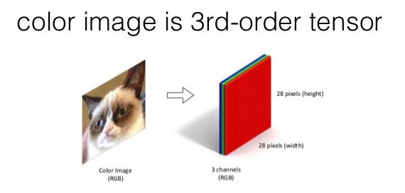
Source: slidesharecdn
10. Convolution and Image Processing
2D Convolution is a very important operation in image processing. It consists of the below steps:
- Start with a small matrix of weights, called a kernel or a filter
- Slide this kernel on the 2D input data, performing element-wise multiplication
- Add the obtained values and put the sum in a single output pixel
The function can seem a bit complex but it’s widely used for performing various image processing operations like sharpening and blurring the images and edge detection. We just need to know the right kernel for the task we are trying to accomplish. Here are a few kernels you can use:
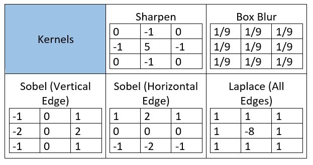
You can download the image I used and try these image processing operations for yourself using the code and the kernels above. Also, try this Computer Vision tutorial on Image Segmentation techniques!
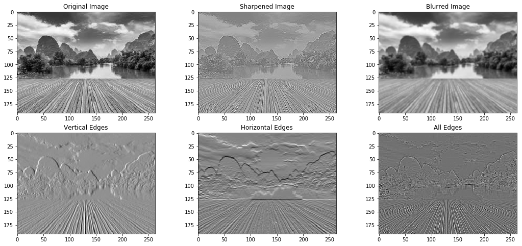
Amazing, right? This is by far my most favorite application of Linear Algebra in Data Science.
Now that you are acquainted with the basics of Computer Vision, it is time to start your Computer Vision journey with 16 awesome OpenCV functions. We also have a comprehensive course on Computer Vision using Deep Learning in which you can work on real-life Computer Vision case studies!
End Notes
My aim here was to make Linear Algebra a bit more interesting than you might have imagined previously. Personally for me, learning about applications of a subject motivates me to learn more about it.
I am sure you are as impressed with these applications as I am. Or perhaps you know of some other applications that I could add to the list? Let me know in the comments section below.


HI Khyati Awesome post keep writing. We need tutors who can make maths easy and fun for ML applications. Thanks Analytics Vidhya for publishing the article. Regards.
Hi Bharat, I am glad you liked the article!
Hello Khyati, Great and very useful reference of the subject. Thanks for sharing. How about articles on calculus and optimization in data science/machine learning?
Hello Hassine, Thank you for your appreciation and for your suggestion. I will try and cover these as well.
Encouraging effort. Keep it up sister
Thank you Syed!