26 minutes
Overview
- The attention mechanism has changed the way we work with deep learning algorithms
- Fields like Natural Language Processing (NLP) and even Computer Vision have been revolutionized by the attention mechanism
- We will learn how this attention mechanism explained works in deep learning, and even implement it in Python
Introduction
“Every once in a while, a revolutionary product comes along that changes everything.” – Steve Jobs
What does one of the most famous quotes of the 21st century have to do with deep learning? Well, think about it. We are in the midst of an unprecedented slew of breakthroughs thanks to advancements in computation power.
And if we had to trace this back to where it began, it would lead us to the Attention Mechanism in deep learning. It is, to put it simply, a revolutionary concept that is changing the way we apply deep learning.
The attention mechanism in NLP is one of the most valuable breakthroughs in Deep Learning research in the last decade. It has spawned the rise of so many recent breakthroughs in natural language processing (NLP), including the Transformer architecture and Google’s BERT
If you’re working in NLP (or want to do so), you simply must know what the Attention mechanism is and how it works.
In this article, we will discuss the basics of several kinds of Attention Mechanisms, how they work, and what the underlying assumptions and intuitions behind them are. We will also provide some mathematical formulations to express the Attention Mechanism completely along with relevant code on how you can easily implement architectures related to Attention in Python.
Table of contents
- What is Attention Mechanism?
- How Attention Mechanism Works?
- How Attention Mechanism was Introduced in Deep Learning
- Implementing a Simple Attention Model in Python Using Keras
- Global vs. Local Attention
- Transformers – Attention is All You Need
- Attention Mechanism in Computer Vision
- Frequently Asked Questions
Quiz Time
Time to dive into the world of Attention Mechanism in Deep Learning! Test your understanding with our quiz! Best of Luck!
What is Attention Mechanism?
Attention mechanisms enhance deep learning models by selectively focusing on important input elements, improving prediction accuracy and computational efficiency. They prioritize and emphasize relevant information, acting as a spotlight to enhance overall model performance.
In psychology, attention is the cognitive process of selectively concentrating on one or a few things while ignoring others.
A neural network is considered to be an effort to mimic human brain actions in a simplified manner. Attention Mechanism is also an attempt to implement the same action of selectively concentrating on a few relevant things, while ignoring others in deep neural networks.
Let me explain what this means. Let’s say you are seeing a group photo of your first school. Typically, there will be a group of children sitting across several rows, and the teacher will sit somewhere in between. Now, if anyone asks the question, “How many people are there?”, how will you answer it?
Simply by counting heads, right? You don’t need to consider any other things in the photo. Now, if anyone asks a different question, “Who is the teacher in the photo?”, your brain knows exactly what to do. It will simply start looking for the features of an adult in the photo. The rest of the features will simply be ignored. This is the ‘Attention’ which our brain is very adept at implementing.
How Attention Mechanism Works?
Here’s how they work:
- Breaking Down the Input: Let’s say you have a bunch of words (or any kind of data) that you want the computer to understand. First, it breaks down this input into smaller pieces, like individual words.
- Picking Out Important Bits: Then, it looks at these pieces and decides which ones are the most important. It does this by comparing each piece to a question or ‘query’ it has in mind.
- Assigning Importance: Each piece gets a score based on how well it matches the question. The higher the score, the more important that piece is.
- Focusing Attention: After scoring each piece, it figures out how much attention to give to each one. Pieces with higher scores get more attention, while less important ones get less attention.
- Putting It All Together: Finally, it adds up all the pieces, but gives more weight to the important ones. This way, the computer gets a clearer picture of what’s most important in the input.
How Attention Mechanism was Introduced in Deep Learning
The attention mechanism emerged as an improvement over the encoder decoder-based neural machine translation system in natural language processing (NLP). Later, this mechanism, or its variants, was used in other applications, including computer vision, speech processing, etc.
Before Bahdanau et al proposed the first Attention model in 2015, neural machine translation was based on encoder-decoder RNNs/LSTMs. Both encoder and decoder are stacks of LSTM/RNN units. It works in the two following steps:
- The encoder LSTM is used to process the entire input sentence and encode it into a context vector, which is the last hidden state of the LSTM/RNN. This is expected to be a good summary of the input sentence. All the intermediate states of the encoder are ignored, and the final state id supposed to be the initial hidden state of the decoder
- The decoder LSTM or RNN units produce the words in a sentence one after another
In short, there are two RNNs/LSTMs. One we call the encoder – this reads the input sentence and tries to make sense of it, before summarizing it. It passes the summary (context vector) to the decoder which translates the input sentence by just seeing it.
The main drawback of this approach is evident. If the encoder makes a bad summary, the translation will also be bad. And indeed it has been observed that the encoder creates a bad summary when it tries to understand longer sentences. It is called the long-range dependency problem of RNN/LSTMs.
RNNs cannot remember longer sentences and sequences due to the vanishing/exploding gradient problem. It can remember the parts which it has just seen. Even Cho et al (2014), who proposed the encoder-decoder network, demonstrated that the performance of the encoder-decoder network degrades rapidly as the length of the input sentence increases.
Although an LSTM is supposed to capture the long-range dependency better than the RNN, it tends to become forgetful in specific cases. Another problem is that there is no way to give more importance to some of the input words compared to others while translating the sentence.
Now, let’s say, we want to predict the next word in a sentence, and its context is located a few words back. Here’s an example – “Despite originally being from Uttar Pradesh, as he was brought up in Bengal, he is more comfortable in Bengali”. In these groups of sentences, if we want to predict the word “Bengali”, the phrase “brought up” and “Bengal”- these two should be given more weight while predicting it. And although Uttar Pradesh is another state’s name, it should be “ignored”.
So is there any way we can keep all the relevant information in the input sentences intact while creating the context vector?
Bahdanau et al (2015) came up with a simple but elegant idea where they suggested that not only can all the input words be taken into account in the context vector, but relative importance should also be given to each one of them.
So, whenever the proposed model generates a sentence, it searches for a set of positions in the encoder hidden states where the most relevant information is available. This idea is called ‘Attention’.
Understanding the Attention Mechanism
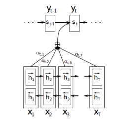
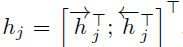
This is the diagram of the Attention model shown in Bahdanau’s paper. The Bidirectional LSTM used here generates a sequence of annotations (h1, h2,….., hTx) for each input sentence. All the vectors h1,h2.., etc., used in their work are basically the concatenation of forward and backward hidden states in the encoder.
To put it in simple terms, all the vectors h1,h2,h3…., hTx are representations of Tx number of words in the input sentence. In the simple encoder and decoder model, only the last state of the encoder LSTM was used (hTx in this case) as the context vector.
But Bahdanau et al put emphasis on embeddings of all the words in the input (represented by hidden states) while creating the context vector. They did this by simply taking a weighted sum of the hidden states.
Now, the question is how should the weights be calculated? Well, the weights are also learned by a feed-forward neural network and I’ve mentioned their mathematical equation below.
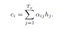
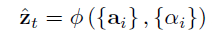
The context vector ci for the output word yi is generated using the weighted sum of the annotations:
The weights αij are computed by a softmax function given by the following equation:
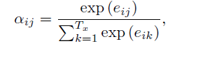
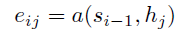
eij is the output score of a feedforward neural network described by the function a that attempts to capture the alignment between input at j and output at i.
Basically, if the encoder produces Tx number of “annotations” (the hidden state vectors) each having dimension d, then the input dimension of the feedforward network is (Tx , 2d) (assuming the previous state of the decoder also has d dimensions and these two vectors are concatenated). This input is multiplied with a matrix Wa of (2d, 1) dimensions (of course followed by addition of the bias term) to get scores eij (having a dimension (Tx , 1)).
On the top of these eij scores, a tan hyperbolic function is applied followed by a softmax to get the normalized alignment scores for output j:
E = I [Tx*2d] * Wa [2d * 1] + B[Tx*1]
α = softmax(tanh(E))
C= IT * α
So, α is a (Tx, 1) dimensional vector and its elements are the weights corresponding to each word in the input sentence.
Let α is [0.2, 0.3, 0.3, 0.2] and the input sentence is “I am doing it”. Here, the context vector corresponding to it will be:
C=0.2*I”I” + 0.3*I”am” + 0.3*I”doing” + + 0.3*I”it” [Ix is the hidden state corresponding to the word x]
Implementing a Simple Attention Model in Python Using Keras
We now have a handle of what this often-quoted Attention mechanism is. Let’s take what we’ve learned and apply it in a practical setting. Yes, let’s get coding!
In this section, we will discuss how a simple Attention model can be implemented in Keras. The purpose of this demo is to show how a simple Attention layer can be implemented in Python.
As an illustration, we have run this demo on a simple sentence-level sentiment analysis dataset collected from the University of California Irvine Machine Learning Repository. You can select any other dataset if you prefer and can implement a custom Attention layer to see a more prominent result.
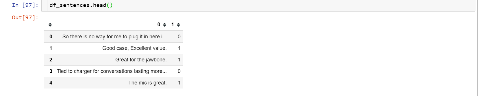
Here, there are only two sentiment categories – ‘0’ means negative sentiment, and ‘1’ means positive sentiment. You’ll notice that the dataset has three files. Among them, two files have sentence-level sentiments and the 3rd one has a paragraph level sentiment.
We are using the sentence level data files (amazon_cells_labelled.txt, yelp_labelled.txt) for simplicity. We have read and merged the two data files. This is what our data looks like:
We then pre-process the data to fit the model using Keras’ Tokenizer() class:
t=Tokenizer()
t.fit_on_texts(corpus)
text_matrix=t.texts_to_sequences(corpus)
The text_to_sequences() method takes the corpus and converts it to sequences, i.e. each sentence becomes one vector. The elements of the vectors are the unique integers corresponding to each unique word in the vocabulary:
len_mat=[]
for i in range(len(text_matrix)):
    len_mat.append(len(text_matrix[i]))
We must identify the maximum length of the vector corresponding to a sentence because typically sentences are of different lengths. We should make them equal by zero padding. We have used a ‘post padding’ technique here, i.e. zeros will be added at the end of the vectors:
from keras.preprocessing.sequence import pad_sequences
text_pad = pad_sequences(text_matrix, maxlen=32, padding='post')
Next, let’s define the basic LSTM based model:
inputs1=Input(shape=(features,))
x1=Embedding(input_dim=vocab_length+1,output_dim=32,\
             input_length=features,embeddings_regularizer=keras.regularizers.l2(.001))(inputs1)
x1=LSTM(100,dropout=0.3,recurrent_dropout=0.2)(x1)
outputs1=Dense(1,activation='sigmoid')(x1)
model1=Model(inputs1,outputs1)
Here, we have used an Embedding layer followed by an LSTM layer. The embedding layer takes the 32-dimensional vectors, each of which corresponds to a sentence, and subsequently outputs (32,32) dimensional matrices i.e., it creates a 32-dimensional vector corresponding to each word. This embedding is also learnt during model training.
Then we add an LSTM layer with 100 number of neurons. As it is a simple encoder-decoder model, we don’t want each hidden state of the encoder LSTM. We just want to have the last hidden state of the encoder LSTM and we can do it by setting ‘return_sequences’= False in the Keras LSTM function.
But in Keras itself the default value of this parameters is False. So, no action is required.
The output now becomes 100-dimensional vectors i.e. the hidden states of the LSTM are 100 dimensional. This is passed to a feedforward or Dense layer with ‘sigmoid’ activation. The model is trained using Adam optimizer with binary cross-entropy loss. The training for 10 epochs along with the model structure is shown below:
model1.summary()
model1.fit(x=train_x,y=train_y,batch_size=100,epochs=10,verbose=1,shuffle=True,validation_split=0.2)
The validation accuracy is reaching up to 77% with the basic LSTM-based model.
Let’s not implement a simple Bahdanau Attention layer in Keras and add it to the LSTM layer. To implement this, we will use the default Layer class in Keras. We will define a class named Attention as a derived class of the Layer class. We need to define four functions as per the Keras custom layer generation rule. These are build(),call (), compute_output_shape() and get_config().
Inside build (), we will define our weights and biases, i.e., Wa and B as discussed previously. If the previous LSTM layer’s output shape is (None, 32, 100) then our output weight should be (100, 1) and bias should be (100, 1) dimensional.
ef build(self,input_shape):
        self.W=self.add_weight(name="att_weight",shape=(input_shape[-1],1),initializer="normal")
        self.b=self.add_weight(name="att_bias",shape=(input_shape[1],1),initializer="zeros")
        super(attention, self).build(input_shape)
Inside call (), we will write the main logic of Attention. We simply must create a Multi-Layer Perceptron (MLP). Therefore, we will take the dot product of weights and inputs followed by the addition of bias terms. After that, we apply a ‘tanh’ followed by a softmax layer. This softmax gives the alignment scores. Its dimension will be the number of hidden states in the LSTM, i.e., 32 in this case. Taking its dot product along with the hidden states will provide the context vector:
def call(self,x):
        et=K.squeeze(K.tanh(K.dot(x,self.W)+self.b),axis=-1)
        at=K.softmax(et)
        at=K.expand_dims(at,axis=-1)
        output=x*at
        return K.sum(output,axis=1)
The above function is returning the context vector. The complete custom Attention class looks like this:
from keras.layers import Layer
import keras.backend as K
class attention(Layer):
def __init__(self,**kwargs):
super(attention,self).__init__(**kwargs)
def build(self,input_shape):
self.W=self.add_weight(name="att_weight",shape=(input_shape[-1],1),initializer="normal")
self.b=self.add_weight(name="att_bias",shape=(input_shape[1],1),initializer="zeros")
super(attention, self).build(input_shape)
def call(self,x):
et=K.squeeze(K.tanh(K.dot(x,self.W)+self.b),axis=-1)
at=K.softmax(et)
at=K.expand_dims(at,axis=-1)
output=x*at
return K.sum(output,axis=1)
def compute_output_shape(self,input_shape):
return (input_shape[0],input_shape[-1])
def get_config(self):
return super(attention,self).get_config()The get_config() method collects the input shape and other information about the model.
Now, let’s try to add this custom Attention layer to our previously defined model. Except for the custom Attention layer, every other layer and their parameters remain the same. Remember, here we should set return_sequences=True in our LSTM layer because we want our LSTM to output all the hidden states.
inputs=Input((features,))
x=Embedding(input_dim=vocab_length+1,output_dim=32,input_length=features,\
            embeddings_regularizer=keras.regularizers.l2(.001))(inputs)
att_in=LSTM(no_of_neurons,return_sequences=True,dropout=0.3,recurrent_dropout=0.2)(x)
att_out=attention()(att_in)
outputs=Dense(1,activation='sigmoid',trainable=True)(att_out)
model=Model(inputs,outputs)
model.summary()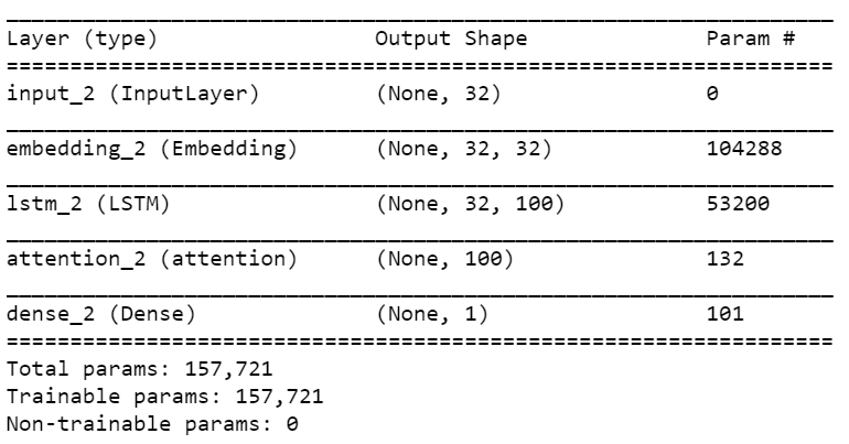
model.compile(loss='binary_crossentropy', optimizer='adam', metrics=['acc'])
model.fit(x=train_x,y=train_y,batch_size=100,epochs=10,verbose=1,shuffle=True,validation_split=0.2)
There is indeed an improvement in the performance as compared to the previous model. The validation accuracy now reaches up to 81.25 % after the addition of the custom Attention layer. With further pre-processing and a grid search of the parameters, we can definitely improve this further.
Different researchers have tried different techniques for score calculation. There are different variants of Attention model(s) according to how the score, as well as the context vector, are calculated. There are other variants also, which we will discuss next.
Global vs. Local Attention
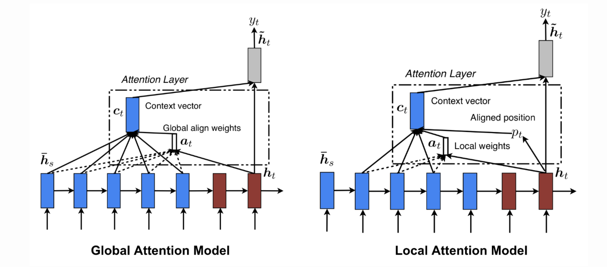
So far, we have discussed the most basic Attention mechanism where all the inputs have been given some importance. Let’s take things a bit deeper now.
The term “global” Attention is appropriate because all the inputs are given importance. Originally, the Global Attention (defined by Luong et al 2015) had a few subtle differences with the Attention concept we discussed previously.
The differentiation is that it considers all the hidden states of both the encoder LSTM and decoder LSTM to calculate a “variable-length context vector ct, whereas Bahdanau et al. used the previous hidden state of the unidirectional decoder LSTM and all the hidden states of the encoder LSTM to calculate the context vector.
In encoder-decoder architectures, the score generally is a function of the encoder and the decoder hidden states. Any function is valid as long as it captures the relative importance of the input words with respect to the output word.
When a “global” Attention layer is applied, a lot of computation is incurred. This is because all the hidden states must be taken into consideration, concatenated into a matrix, and multiplied with a weight matrix of correct dimensions to get the final layer of the feedforward connection.
So, as the input size increases, the matrix size also increases. In simple terms, the number of nodes in the feedforward connection increases and in effect it increases computation.
Can we reduce this in any way? Yes! Local Attention is the answer.
Intuitively, when we try to infer something from any given information, our mind tends to intelligently reduce the search space further and further by taking only the most relevant inputs.
The idea of Global and Local Attention was inspired by the concepts of Soft and Hard Attention used mainly in computer vision tasks.
Soft Attention is the global Attention where all image patches are given some weight; but in hard Attention, only one image patch is considered at a time.
But local Attention is not the same as the hard Attention used in the image captioning task. On the contrary, it is a blend of both the concepts, where instead of considering all the encoded inputs, only a part is considered for the context vector generation. This not only avoids expensive computation incurred in soft Attention but is also easier to train than hard Attention.
How can this be achieved in the first place? Here, the model tries to predict a position pt in the sequence of the embeddings of the input words. Around the position pt, it considers a window of size, say, 2D. Therefore, the context vector is generated as a weighted average of the inputs in a position [pt – D,pt + D] where D is empirically chosen.
Furthermore, there can be two types of alignments:
- Monotonic alignment, where pt is set to t, assuming that at time t, only the information in the neighborhood of t matters
- Predictive alignment where the model itself predicts the alignment position as follows:
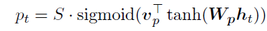
where ‘Vp’ and ‘Wp’ are the model parameters that are learned during training and ‘S’ is the source sentence length. Clearly, pt ε [0,S].
The figures below demonstrate the difference between the Global and Local Attention mechanism. Global Attention considers all hidden states (blue) whereas local Attention considers only a subset:
Transformers – Attention is All You Need
The paper named “Attention is All You Need” by Vaswani et al is one of the most important contributions to Attention so far. They have redefined Attention by providing a very generic and broad definition of Attention based on key, query, and values. They have referenced another concept called multi-headed Attention. Let’s discuss this briefly.
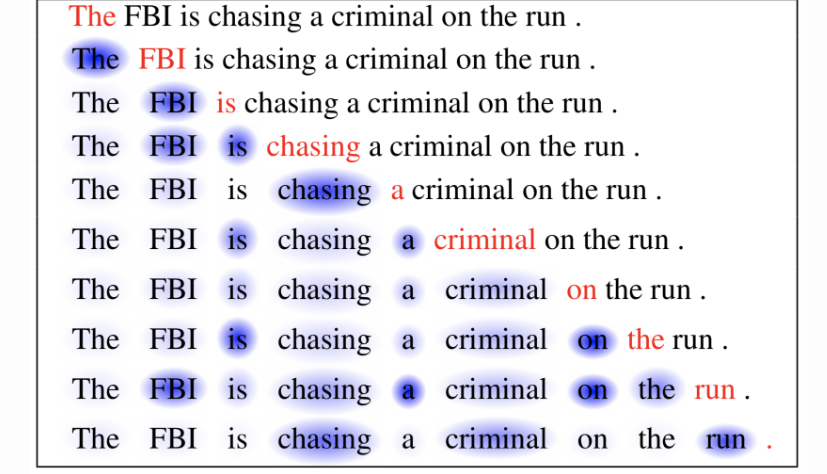
First, let’s define what “self-Attention” is. Cheng et al, in their paper named “Long Short-Term Memory-Networks for Machine Reading”, defined self-Attention as the mechanism of relating different positions of a single sequence or sentence in order to gain a more vivid representation.
Machine reader is an algorithm that can automatically understand the text given to it. We have taken the below picture from the paper. The red words are read or processed at the current instant, and the blue words are the memories. The different shades represent the degree of memory activation.
When we are reading or processing the sentence word by word, where previously seen words are also emphasized on, is inferred from the shades, and this is exactly what self-Attention in a machine reader does.
Previously, to calculate the Attention for a word in the sentence, the mechanism of score calculation was to either use a dot product or some other function of the word with the hidden state representations of the previously seen words. In this paper, a fundamentally same but a more generic concept altogether has been proposed.
Let’s say we want to calculate the Attention for the word “chasing”. The mechanism would be to take a dot product of the embedding of “chasing” with the embedding of each of the previously seen words like “The”, “FBI”, and “is”.
Now, according to the generalized definition, each embedding of the word should have three different vectors corresponding to it, namely Key, Query, and Value. We can easily derive these vectors using matrix multiplications.
Whenever we are required to calculate the Attention of a target word with respect to the input embeddings, we should use the Query of the target and the Key of the input to calculate a matching score, and these matching scores then act as the weights of the Value vectors during summation.
Now, you might ask what these Key, Query and Value vectors are. These are basically abstractions of the embedding vectors in different subspaces. Think of it in this way: you raise a query; the query hits the key of the input vector. The Key can be compared with the memory location read from, and the value is the value to be read from the memory location. Simple, right?
If the dimension of the embeddings is (D, 1) and we want a Key vector of dimension (D/3, 1), we must multiply the embedding by a matrix Wk of dimension (D/3, D). So, the key vector becomes K=Wk*E. Similarly, for Query and Value vectors, the equations will be Q=Wq*E, V=Wv*E (E is the embedding vector of any word).
Now, to calculate the Attention for the word “chasing”, we need to take the dot product of the query vector of the embedding of “chasing” to the key vector of each of the previous words, i.e., the key vectors corresponding to the words “The”, “FBI” and “is”. Then these values are divided by D (the dimension of the embeddings) followed by a softmax operation. So, the operations are respectively:
- softmax(Q”chasing” . K”The” / D)
- softmax(Q”chasing” .K”FBI” / D)
- softmax(Q”chasing” . K”is” / D)
Basically, this is a function f(Qtarget, Kinput) of the query vector of the target word and the key vector of the input embeddings. It doesn’t necessarily have to be a dot product of Q and K. Anyone can choose a function of his/her own choice.
Next, let’s say the vector thus obtained is [0.2, 0.5, 0.3]. These values are the “alignment scores” for the calculation of Attention. These alignment scores are multiplied with the value vector of each of the input embeddings and these weighted value vectors are added to get the context vector:
C”chasing”= 0.2 * VThe + 0.5* V”FBI” + 0.3 * V”is”
Practically, all the embedded input vectors are combined in a single matrix X, which is multiplied with common weight matrices Wk, Wq, Wv to get K, Q and V matrices respectively. Now the compact equation becomes:
Z=Softmax(Q*KT/D)V
Therefore, the context vector is a function of Key, Query and Value F(K, Q, V).
The Bahdanau Attention or all other previous works related to Attention are the special cases of the Attention Mechanisms described in this work. The salient feature/key highlight is that the single embedded vector is used to work as Key, Query and Value vectors simultaneously.
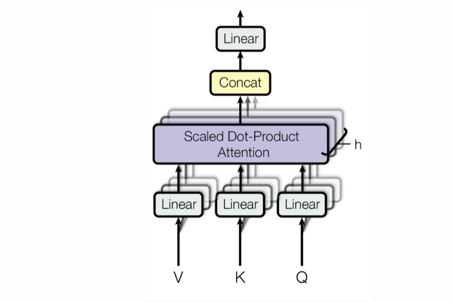
In multi-headed Attention, matrix X is multiplied by different Wk, Wq and Wv matrices to get different K, Q and V matrices respectively. And we end up with different Z matrices, i.e., embedding of each input word is projected into different “representation subspaces”.
In, say, 3-headed self-Attention, corresponding to the “chasing” word, there will be 3 different Z matrices also called “Attention Heads”. These Attention heads are concatenated and multiplied with a single weight matrix to get a single Attention head that will capture the information from all the Attention heads.
The picture below depicts the multi-head Attention. You can see that there are multiple Attention heads arising from different V, K, Q vectors, and they are concatenated:
The actual transformer architecture is a bit more complicated. You can read it in much more detail here.
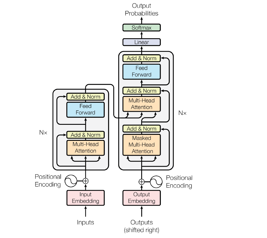
This image above is the transformer architecture. We see that something called ‘positional encoding’ has been used and added with the embedding of the inputs in both the encoder and decoder.
The models that we have described so far had no way to account for the order of the input words. They have tried to capture this through positional encoding. This mechanism adds a vector to each input embedding, and all these vectors follow a pattern that helps to determine the position of each word, or the distances between different words in the input.
As shown in the figure, on top of this positional encoding + input embedding layer, there are two sublayers:
- In the first sublayer, there is a multi-head self-attention layer. There is an additive residual connection from the output of the positional encoding to the output of the multi-head self-attention, on top of which they have applied a layer normalization layer. The layer normalization is a technique (Hinton, 2016) similar to batch normalization where instead of considering the whole minibatch of data for calculating the normalization statistics, all the hidden units in the same layer of the network have been considered in the calculations. This overcomes the drawback of estimating the statistics for the summed input to any neuron over a minibatch of the training samples. Thus, it is convenient to use in RNN/LSTM.
- In the second sublayer, instead of the multi-head self-attention, there is a feedforward layer (as shown), and all other connections are the same.
On the decoder side, apart from the two layers described above, there is another layer that applies multi-head Attention on top of the encoder stack. Then, after a sublayer followed by one linear and one softmax layer, we get the output probabilities from the decoder.
Attention Mechanism in Computer Vision
You can intuitively understand where the Attention mechanism can be applied in the NLP space. We want to explore beyond that. So in this section, let’s discuss the Attention mechanism in the context of computer vision. We will reference a few key ideas here, and you can explore more in the papers we have referenced.
Image Captioning-Show, Attend and Tell (Xu et al, 2015):
In image captioning, a convolutional neural network is used to extract feature vectors known as annotation vectors from the image. This produces L number of D dimensional feature vectors, each of which is a representation corresponding to a part of an image.
In this work, features have been extracted from a lower convolutional layer of the CNN model so that a correspondence between the extracted feature vectors and the portions of the image can be determined. On top of this, an Attention mechanism is applied to selectively give more importance to some of the locations of the image compared to others, for generating caption(s) corresponding to the image.
A slightly modified version of Bahdanau Attention has been used here. Instead of taking a weighted sum of the annotation vectors (similar to hidden states explained earlier), a function has been designed that takes both the set of annotation vectors and the alignment vector, and outputs a context vector instead of simply creating a dot product (mentioned above).
Although this work by Google DeepMind is not directly related to Attention, this mechanism has been ingeniously used to mimic the way an artist draws a picture. This is done by drawing parts of the image sequentially.
Let’s discuss this paper briefly to get an idea about how this mechanism alone or combined with other algorithms can be used intelligently for many interesting tasks.
The main idea behind this work is to use a variational autoencoder for image generation. Unlike a simple autoencoder, a variational autoencoder does not generate the latent representation of a data directly. Instead, it generates multiple Gaussian distributions (say N number of Gaussian distributions) with different means and standard deviations.
From these N number of Gaussian distributions, an N element latent vector is sampled, and this sample is fed to the decoder for the output image generation. Note that Attention-based LSTMs have been used here for both encoder and decoder of the variational autoencoder framework.
But what is that?
The main intuition behind this is to iteratively construct an image. At every time step, the encoder passes one new latent vector to the decoder and the decoder improves the generated image in a cumulative fashion, i.e. the image generated at a certain time step gets enhanced in the next timestep. It is like mimicking an artist’s act of drawing an image step by step.
But the artist does not work on the entire picture at the same time, right?. He/she does it in parts – if he is drawing a portrait, at an instant he/she does not draw the ear, eyes or other parts of a face together. He/she finishes drawing the eye and then moves on to another part.
If we use a simple LSTM, it will not be possible to focus on a certain part of an image at a certain time step. Here is how Attention becomes relevant.
At both the encoder and decoder LSTM, one Attention layer (named “Attention gate”) has been used. So, while encoding or “reading” the image, only one part of the image gets focused on at each time step. And similarly, while writing, only a certain part of the image gets generated at that time-step.
Conclusion
This was quite a comprehensive look at the popular Attention mechanism and how it applies to deep learning. I’m sure you must have gathered why this has made quite a dent in the deep learning space. It is extraordinarily effective and has already penetrated multiple domains.
This Attention mechanism has uses beyond what we mentioned in this article. If you have used it in your role or any project, we would love to hear from you. Let us know in the comments section below and we’ll connect! Hope you like this article and get understanding about the attention mechanism explained, and attention model.
Frequently Asked Questions
Q1. What is the attention mechanism in deep learning?
A. Attention mechanisms is a layer of neural networks added to deep learning models to focus their attention to specific parts of data, based on different weights assigned to different parts.
Q2. What is the difference between global and local attention?
A. Global attention means that the model is attending to all the available data. In local attention, the model focuses on only certain subsets of the entire data.
Q3. What are the two types of attention mechanisms?
A. There are two types of attention mechanisms: additive attention and dot-product attention. Additive attention computes the compatibility between the query and key vectors using a feed-forward neural network, while dot-product attention measures their similarity using dot product.
Q4. What is attention mechanism in machine translation?
A. In machine translation, attention mechanism is used to align and selectively focus on relevant parts of the source sentence during the translation process. It allows the model to assign weights to more important words or phrases.
Q5. What are Transformer and attention mechanisms?
A. The Transformer is a neural network architecture that relies heavily on attention mechanisms. It uses self-attention to capture dependencies between words in an input sequence, allowing it to model long-range dependencies more effectively than traditional recurrent neural networks.


thanks for the article, please publish your code.
Hi Thanks for sharing such a great post. It's really informative and easy to read.
Thanks Pradip and Sayan for sharing this!
I need help for attention code please, I executed the code, but I had a problem of ( train_x and train_y ) values. Any help please.
Hi, Great article! One question, How to add regularization element to the Attention layer viz. kernel_regularization or DropAttention?
Several variables are not defined or imported anywhere in the code you provided, so please make the code runnable.
Thank you. It was so helpful. Could you please guide me on how can I get rid of local minima in a transformer network?
Explained in a very simplified yet useful manner...Thanks
Thank you for the article, very helpful. Yet, I couldn't test the example of the sentence level sentiment analysis. Can you publish the code please?
Hi, Thanks for the great post. BTW I got error in Keras backend squeeze function: Dict not callable et=K.squeeze(tanh,axis=-1) TypeError: 'dict' object is not callable Call arguments received: • x=tf.Tensor(shape=(None, 119, 100), dtype=float32)
Solved a lot of my confusion, thank you for sharing!