A Unique Method for Machine Learning Interpretability: Game Theory & Shapley Values!
Overview
- Learn how to use Shapley values in game theory for machine learning interpretability
- It’s a unique and different perspective to interpret black-box machine learning models
Introduction
Let’s roll back the time to 2007 when the first-ever cricket T20 World Cup was organized. The world was harping about it but the cricket associations were looking at it with caution – the commercial breaks were reduced from 99 seconds to 39 seconds. Ouch! That’s quite a bit of a reduction in revenue.
But this decision was the most rewarding one in the long run, and now its the highest revenue grossing format in the history of cricket!
The world will be taken by storm by the Indian Cricket Team at the T-20 World Cup in 2020! Our captain Virat Kohli will once again be in the spotlight for taking critical decisions. Isn’t that a very stressful job? Especially when the hopes of millions of people dwell upon you?

Wait – what does all of this have to do with machine learning interpretability, Shapley values, and Game Theory? Here’s a thought to put things into context:
What if we can build an interesting decision theory to support all the key decisions with utmost accuracy? That would be wonderful, right? It could simply solve all the confusion, like – the first batsmen to send for batting, the bowler to be chosen, the field placement, etc.
We can do this with the application of Game Theory! So in this article, we will further explore an alternative method of interpreting Machine Learning models which stems out of the game theory discipline. We will introduce and talk about Shapley Values for machine learning interpretability.
Well, it is alright if you do not have even basic level exposure to Game Theory. I will cover the basics required and without digressing will focus on a concept called Shapley values and how that can help to interpret machine learning models with an implementation in Python using the SHAP library.
Table of Contents
- What Is Game Theory?
- Cooperative Game Theory
- Shapley Values: Intuition
- Shapley Values for Machine Learning Interpretability
- Model Interpretation using SHAP in Python
- Global Interpretation using Shapley Values
What Is Game Theory?
Let’s define Game Theory first before we get into the crux of this article. This will hold us in good stead as we dive into the way Game Theory is used for interpreting machine learning models.
Game theory is a theoretical framework for social situations among competing players. It is the science of optimal decision-making of independent and competing actors in a strategic setting.
The key pioneers of game theory were mathematicians John von Neumann and John Nash, as well as economist Oskar Morgenstern.
Now, you might be asking – what is a game? Is it like chess? Video Games?
A “Game” is any situation in which there are several decision-makers, and each of them wants to optimize their results. The optimizing decision will depend on the decisions of others. The game identifies the players’ identities, preferences, and available strategies and how these strategies affect the outcome.
Game Theory attempts to define these situations in mathematical terms and determine what would happen if every player acts rationally.
- Perhaps an equilibrium can be reached (which is why we all drive on the same side of the road within a country)
- Maybe this equilibrium will be worse for all players (which is why people litter or pollute common resources)
- Well, everyone will try to be as unpredictable as possible in their actions (as might happen with troop deployment in a war)
In essence, Game Theory is a way to mathematically model complex human behavior, to try to understand it, and predict it. You can read more about game theory and it’s fit in the AI world in this excellent and detailed walkthrough. It’s a fascinating concept!
Cooperative Game Theory
Cooperative game theory assumes that groups of players, called coalitions, are the primary units of decision-making, and may enforce cooperative behavior.
Consequently, cooperative games can be seen as a competition between coalitions of players, rather than between individual players.

Let’s try to understand cooperative game theory using the concept of Shapley values.
The Intuition behind Shapley Values
I love learning any new concept using illustrations and examples so that’s exactly what we’ll do here.
Let’s first design a cooperative game. Three friends – Ram, Abhiraj, and Pranav – go out for a meal. They order and share fries, wine, and pi. It is hard to figure out who should pay how much since they did not eat an equal share. So, we have the following information:
- If Ram is eating alone, he would pay 800
- If Abhiraj is eating alone, he would pay 560
- If Pranav is eating alone, he would pay 700
- If Ram and Abhiraj both eat alone, they would pay 800
- If Ram and Pranav both eat alone, they would pay 850
- If Abhiraj and Pranav both eat alone, they would pay 720
- If Ram, Abhiraj, and Pranav all eat together, they would pay 900

So, it turns out the actual amount all 3 of them pay when they eat together is 900. Now, the task at hand is to figure out how much each of them should pay individually.
The method we will adapt here is:
We take all permutations of the 3 participants in sequence and see the incremental payout that each of them has to make.
So here, the sequence is Ram, Abhiraj and then Pranav in turn. As described above, Ram comes and pays 800. Now, Ram and Abhiraj pay 800 only so there is no additional payout for Abhiraj. Hence, we get 0. And finally, all 3 eat together and pay 900 so the additional payout for Pranav is 100.
We repeat the same exercise for each possible order for the 3 friends and get the following marginal payout values:
- (Ram, Abhiraj, Pranav) – (800,0,100)
- (Abhiraj, Ram, Pranav) – (560, 240, 100)
- (Abhiraj, Pranav, Ram) – (560, 160, 180)
- (Pranav, Ram, Abhiraj) – (700, 150, 50)
- (Pranav, Abhiraj, Ram) – (700, 20, 180)
- (Ram, Pranav, Abhiraj) – (800, 50, 50)
So, what is the Shapley value for Ram, Abhiraj, and Pranav each? It is just the average of the marginal payout for each!
For example, for Ram it is (800 + 240 + 180 + 150 + 180 + 800)/6 = 392. Similarly, for Abhiraj it is 207, and for Pranav, it turns out to be 303. The total turns out to be 900.
So now we have reached to the final amount that each of them should pay if all 3 go out together. In the next section, we will see how we can use the concept of Shapley values to interpret machine learning models.
Shapley Values for Machine Learning Interpretability
You have an intuition behind what Shapley values are – so take a moment to think about how they could help in interpreting a black-box machine learning model.
We know that each value of an independent variable or a feature for a given sample is a part of a cooperative game where we assume that prediction is actually the payout. So, let us dive into another example to understand this in detail.
Assume the following scenario:
We have trained a machine learning model to predict house prices in Delhi. For a certain house, our model predicts INR 51,00,000 and we need to explain this prediction. The apartment has a size of 50 yards, has a private pool and also a garage:

The average prediction for all apartments is INR 50,00,000. How much has each feature value contributed to the prediction compared to the average prediction?
Now, if we talk in terms of Game Theory, the “game” here is the prediction task for a single instance of the dataset. The “players” are the feature values of the instance that collaborate to play the game (predict a value) similar to the meal example where Pranav, Ram, and Abhiraj went for a meal together.
In our house example, the feature values has_pool, has_garageand area-50 worked together to achieve the prediction of INR 51,00,000. Our goal is to explain the difference between the actual prediction (INR 51,00,000) and the average prediction (50,00,000): a difference of INR 1,00,000.
A possible explanation could be has_pool contributed INR 30,000, garage contributed INR 50,000, and area of 50 yards contributed INR 20,000. The contributions add up to INR 1,00,000 – the final prediction minus the average predicted house price.
To summarise, the Shapley value for each variable (payout) is basically trying to find the correct weight such that the sum of all Shapley values is the difference between the predictions and average value of the model. In other words, Shapley values correspond to the contribution of each feature towards pushing the prediction away from the expected value.
Now that we have understood the underlying intuition for Shapley values and how useful they can be in interpreting machine learning models, let us look at its implementation in Python.
Model Interpretation using SHAP in Python
The SHAP library in Python has inbuilt functions to use Shapley values for interpreting machine learning models. It has optimized functions for interpreting tree-based models and a model agnostic explainer function for interpreting any black-box model for which the predictions are known.
In the model agnostic explainer, SHAP leverages Shapley values in the below manner. To get the importance of feature X{i}:
- Get all subsets of features S that do not contain X{i}
- Compute effect on our predictions of adding X{i} to all those subsets
- Aggregate all contributions to compute the marginal contribution of the feature
Now, for these subsets, SHAP does not go on and retrain the model for each subset. Instead, for the removed or left out feature, it just replaces it with the average value of the feature and generates the predictions.
It’s now time to work on a real dataset! As we did in the previous article, we will use the Big Mart Sales problem hosted on our Datahack Platform.
The problem statement is about predicting sales for different items being sold at different outlets. You can download the dataset from the above link. We will use Shapley values and also go through some visualizations to look at both local and global interpretations.
Note: You can go through this course to fully understand how to build models using this data. Our focus here is to narrow down on the Shapley value interpretability part.
You can install the SHAP library using the terminal command:
conda install -c conda-forge shap
Now, let’s begin with building a model for predicting sales. First, we will import the necessary libraries:
# importing the required libraries
import pandas as pd
import numpy as np
import shap
from sklearn.model_selection import train_test_split
from sklearn.metrics import mean_squared_error

from sklearn.linear_model import LinearRegression
from sklearn.tree import DecisionTreeRegressor
from sklearn.ensemble import RandomForestRegressor
from xgboost.sklearn import XGBRegressor
from sklearn.preprocessing import OneHotEncoder, LabelEncoder
from sklearn import tree

import matplotlib.pyplot as plt
%matplotlib inline
import warnings
warnings.filterwarnings('ignore')
Reading Data
# reading the data
df = pd.read_csv('data.csv')
Missing Value Treatment
# imputing missing values in Item_Weight by median and Outlet_Size with mode
df['Item_Weight'].fillna(df['Item_Weight'].median(), inplace=True)
df['Outlet_Size'].fillna(df['Outlet_Size'].mode()[0], inplace=True)
Feature Engineering
Python Code:
Data Preprocessing
# label encoding the ordinal variables
le = LabelEncoder()
df['Outlet'] = le.fit_transform(df['Outlet_Identifier'])
var_mod = ['Item_Fat_Content','Outlet_Location_Type','Outlet_Size','Item_Type_Combined','Outlet_Type','Outlet']
le = LabelEncoder()
for i in var_mod:
df[i] = le.fit_transform(df[i])

# one hot encoding the remaining categorical variables
df = pd.get_dummies(df, columns=['Item_Fat_Content','Outlet_Location_Type','Outlet_Size','Outlet_Type',
                              'Item_Type_Combined','Outlet'])
Train-Test Split
# dropping the ID variables and variables that have been used to extract new variables
df.drop(['Item_Type','Outlet_Establishment_Year', 'Item_Identifier', 'Outlet_Identifier'],axis=1,inplace=True)

# separating the dependent and independent variables
X = df.drop('Item_Outlet_Sales',1)
y = df['Item_Outlet_Sales']

# creating the training and validation set
X_train, X_test, y_train, y_test = train_test_split(X, y, test_size=.25, random_state=42)
Initialize Shap
# Need to load JS vis in the notebook
shap.initjs()
Fitting XGBoost
xgb_model = XGBRegressor(n_estimators=1000, max_depth=10, learning_rate=0.001, random_state=0)
xgb_model.fit(X_train, y_train)
Generating Predictions
y_predict = xgb_model.predict(X_test)
Evaluating Performance
mean_squared_error(y_test, y_predict)**(0.5)
Local Interpretation using SHAP (for prediction at id number 4776)
explainer = shap.TreeExplainer(xgb_model)
shap_values = explainer.shap_values(X_train)
i = 4776
shap.force_plot(explainer.expected_value, shap_values[i], features=X_train.loc[4776], feature_names=X_train.columns)
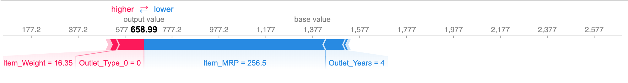
In blue, we have negative Shap values that show everything that pushes the sales value in the negative direction. While the Shap value in red represents everything that pushes it towards a positive direction. Note that this is only for observation number 4776.
Next, let us look at a function that can generate a neat summary for us.
Global Interpretation using Shapley values
Now that we can calculate Shap values for each feature of every observation, we can get a global interpretation using Shapley values by looking at it in a combined form. Let’s see how we can do that:
shap.summary_plot(shap_values, features=X_train, feature_names=X_train.columns)
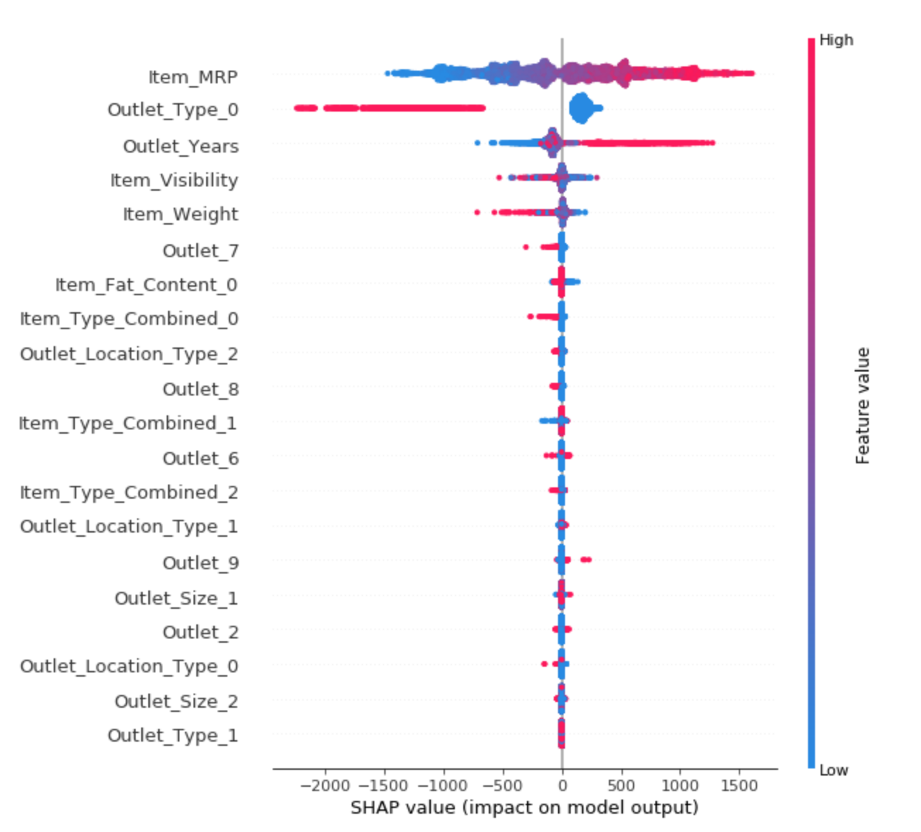
We get the above plot by putting everything together under one roof. This shows the Shap values on the x-axis. Here, all the values on the left represent the observations that shift the predicted value in the negative direction while the points on the right contribute to shifting the prediction in a positive direction. All the features are on the left y-axis.
So here, high MRP values are on the right side primarily because they contribute positively to the sales value for each item. Similarly, for outlets with outlet type 0, they have a high impact on pushing the item sales in the negative direction.
End Notes
Interpretability remains a very important aspect of machine learning and data science as more complex models are brought into production. LIME and Shapley are two such methods that have started seeing some adoption in the industry.
With the advent of deep learning, there is more research being done on how to interpret Natural Language Processing (NLP) and computer vision models. The interpretability aspect of computer vision has been covered to some extent
I hope this was a helpful read for you. Please share your views in the comments section below!
IIT Bombay Graduate with a Masters and Bachelors in Electrical Engineering. I have previously worked as a lead decision scientist for Indian National Congress deploying statistical models (Segmentation, K-Nearest Neighbours) to help party leadership/Team make data-driven decisions. My interest lies in putting data in heart of business for data-driven decision making.


Hi, this line (Ram, Pranav, Abhiraj) – (800, 50, 900) should have been (Ram, Pranav, Abhiraj) – (800, 50, 50) for what I understood, right?
Yes, that is a typo. Thanks for notifying :)
Generally, we will be doing predictions on the test data and in this case would like to know if the below modification is correct ? i = 1 shap.force_plot(explainer.expected_value, shap_values[i], features=X_test.loc[1], feature_names=X_train.columns)
hi, I want to know why we explain the model on X_train, should it be X_test? what is the right approach?