Build your first Machine Learning pipeline using scikit-learn!
Overview
- Understand the structure of a Machine Learning Pipeline
- Build an end-to-end ML pipeline on a real-world data
- Train a Random Forest Regressor for sales prediction
Introduction
For building any machine learning model, it is important to have a sufficient amount of data to train the model. The data is often collected from various resources and might be available in different formats. Due to this reason, data cleaning and preprocessing become a crucial step in the machine learning project.
Whenever new data points are added to the existing data, we need to perform the same preprocessing steps again before we can use the machine learning model to make predictions. This becomes a tedious and time-consuming process!

An alternate to this is creating a machine learning pipeline that remembers the complete set of preprocessing steps in the exact same order. So that whenever any new data point is introduced, the machine learning pipeline performs the steps as defined and uses the machine learning model to predict the target variable.
This is exactly what we are going to cover in this article – design a machine learning pipeline and automate the iterative processing steps.
Table of Contents
- Understanding Problem Statement
- Building a prototype model
- Data Exploration and Preprocessing
- Impute the missing values
- Encode the categorical variables
- Normalize/Scale the data if required
- Model Building
- Identifying features to predict the target
- Data Exploration and Preprocessing
- Designing the ML Pipeline using the best model
- Predict the target on the unseen data.
Understanding Problem Statement
In order to make the article intuitive, we will learn all the concepts while simultaneously working on a real world data – BigMart Sales Prediction.
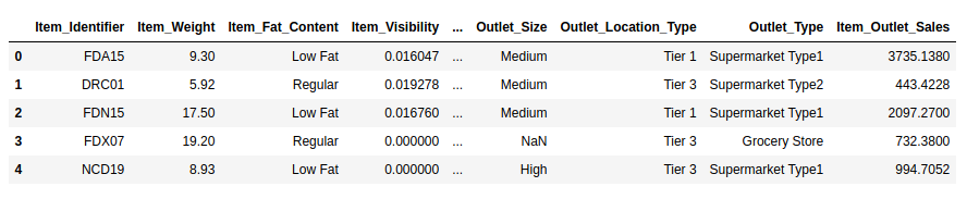
As a part of this problem, we are provided with the information about the stores (location, size, etc), products (weight, category, price, etc) and historical sales data. Using this information, we have to forecast the sales of the products in the stores.
You can read the detailed problem statement and download the dataset from here. Below is the complete set of features in this data.The target variable here is the Item_Outlet_Sales.
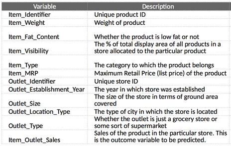
I encourage you to go through the problem statement and data description once before moving to the next section so that you have a fair understanding of the features present in the data.
Building a prototype model
To build a machine learning pipeline, the first requirement is to define the structure of the pipeline. In other words, we must list down the exact steps which would go into our machine learning pipeline.
In order to do so, we will build a prototype machine learning model on the existing data before we create a pipeline. The main idea behind building a prototype is to understand the data and necessary preprocessing steps required before the model building process. Based on our learning from the prototype model, we will design a machine learning pipeline that covers all the essential preprocessing steps.
The focus of this section will be on building a prototype that will help us in defining the actual machine learning pipeline for our sales prediction project. Let’s get started!
Data Exploration and Preprocessing
What is the first thing you do when you are provided with a dataset? You would explore the data, go through the individual variables, and clean the data to make it ready for the model building process.
That is exactly what we will be doing here. We will explore the variables and find out the mandatory preprocessing steps required for the given data. Let us start by checking if there are any missing values in the data. We will use the isnull().sum() function here
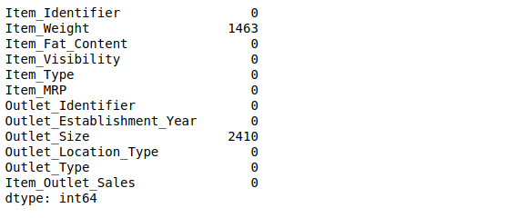
There are only two variables with missing values – Item_Weight and Outlet_Size.
Since Item_Weight is a continuous variable, we can use either mean or median to impute the missing values. On the other hand, Outlet_Size is a categorical variable and hence we will replace the missing values by the mode of the column. You can try different methods to impute missing values as well.
Have you built any machine learning models before? If yes, then you would know that most machine learning models cannot handle missing values on their own. Thus imputing missing values becomes a necessary preprocessing step.
Additionally, machine learning models cannot work with categorical (string) data as well, specifically scikit-learn. Before building a machine learning model, we need to convert the categorical variables into numeric types. Let us do that.
Encode the categorical variables
To check the categorical variables in the data, you can use the train_data.dtypes() function. This will give you a list of the data types against each variable. For the BigMart sales data, we have the following categorical variable –
- Item_Fat_Content
- Item_Type, Outlet_Identifier
- Outlet_Size, Outlet_Location_Type, and
- Outlet_Type
There are a number of ways in which we can convert these categories into numerical values. You can read about the same in this article – Simple Methods to deal with Categorical Variables. We are going to use the categorical_encoders library in order to convert the variables into binary columns.
Note that in this example I am not going to encode Item_Identifier since it will increase the number of feature to 1500. This feature can be used in other ways (read here), but to keep the model simple, I will not use this feature here.
Scale the data:
So far we have taken care of the missing values and the categorical (string) variables in the data. Next we will work with the continuous variables. Often the continuous variables in the data have different scales, for instance, a variable V1 can have a range from 0 to 1 while another variable can have a range from 0-1000.
Based on the type of model you are building, you will have to normalize the data in such a way that the range of all the variables is almost similar. You can do this easily in python using the StandardScaler function.
Model Building
Now that we are done with the basic pre-processing steps, we can go ahead and build simple machine learning models over this data. We will try two models here – Linear Regression and Random Forest Regressor to predict the sales.
To compare the performance of the models, we will create a validation set (or test set). Here I have randomly split the data into two parts using the train_test_split() function, such that the validation set holds 25% of the data points while the train set has 75%
![]()
Great, we have our train and validation sets ready. Let us train a linear regression model on this data and check it’s performance on the validation set. To check the model performance, we are using RMSE as an evaluation metric.
Note: If you are not familiar with Linear regression, you can go through the article below-

The linear regression model has a very high RMSE value on both training and validation data. Let us see if a tree-based model performs better in this case. Here we will train a random forest and check if we get any improvement in the train and validation errors.
Note: To learn about the working of Random forest algorithm, you can go through the article below-

As you can see, there is a significant improvement on is the RMSE values. You can train more complex machine learning models like Gradient Boosting and XGBoost, and see of the RMSE value further improves.
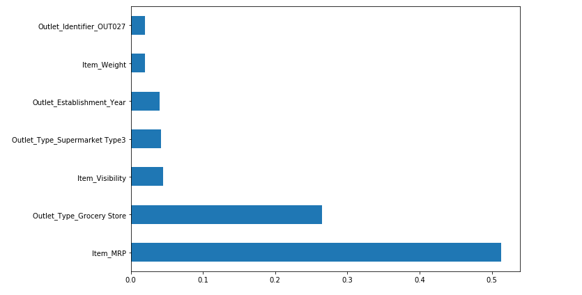
A very interesting feature of the random forest algorithm is that it gives you the ‘feature importance’ for all the variables in the data. Let us see how can we use this attribute to make our model simpler and better!
Feature Importance
After the preprocessing and encoding steps, we had a total of 45 features and not all of these may be useful in forecasting the sales. Alternatively we can select the top 5 or top 7 features, which had a major contribution in forecasting sales values.
If the model performance is similar in both the cases, that is – by using 45 features and by using 5-7 features, then we should use only the top 7 features, in order to keep the model more simple and efficient.
The idea is to have a less complex model without compromising on the overall model performance.
Following is the code snippet to plot the n most important features of a random forest model.
Now, we are going to train the same random forest model using these 7 features only and observe the change in RMSE values for the train and the validation set.

Now, this is amazing! Using only 7 features has given almost the same performance as the previous model where we were using 45 features. Let us identify the final set of features that we need and the preprocessing steps for each of them.
Identifying features to build the ML pipeline
As discussed initially, the most important part of designing a machine leaning pipeline is defining its structure, and we are almost there!
We are now familiar with the data, we have performed required preprocessing steps, and built a machine learning model on the data. At this stage we must list down the final set of features and necessary preprocessing steps (for each of them) to be used in the machine learning pipeline.
Selected Features and Preprocessing Steps
- Item_MRP: It holds the price of the products. During the preprocessing step we used a standard scaler to scale this values.
- Outlet_Type_Grocery_Store: A binary column which indicates if the outlet type is a grocery store or not. To use this information in the model building process, we will add a binary feature in the existing data that contains 1 (if outlet type is a grocery store) and 0 ( if outlet type is something else).
- Item_Visibility: Denotes visibility of products in the store. Since this variable had a small value range and no missing values, we didn’t apply any preprocessing steps on this variable.
- Outlet_Type_Supermarket_Type3: Another binary column indicating if the outlet type is a “supermarket_type_3” or not. To capture this information we will create binary feature that stores 1 (if outlet type is supermarket_type_3) and 0 (othewise).
- Outlet_Identifier_OUT027: This feature specifies whether the outlet identifier is “OUT027” or not. Similar to the last previous example, we will create a separate column that carries 1 (if outlet type is grocery store) and 0 (otherwise).
- Outlet_Establishment_Year: The Outlet_Establishment_Year describes year of establishment of the stores. Since we did not perform any transformation on values in this column, we will not preprocess it in the pipeline as well.
- Item_Weight: During the preprocessing steps we observed that Item_Weight had missing values. These missing values were imputed using the average of the column. This has to be taken into account while building the machine learning pipeline.
Apart from these 7 columns, we will drop the rest of the columns since we will not use them to train the model. Let us go ahead and design our ML pipeline!
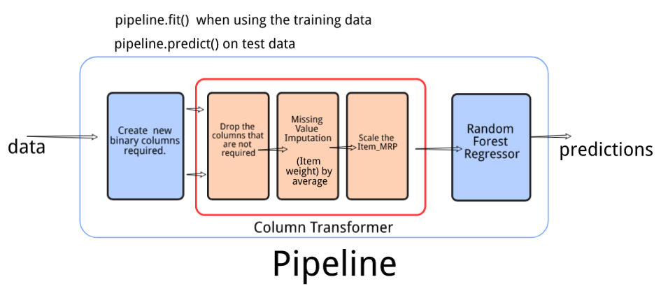
Pipeline Design
In the last section we built a prototype to understand the preprocessing requirement for our data. It is now time to form a pipeline design based on our learning from the last section. We will define our pipeline in three stages:
- Create the required binary features
- Perform required data preprocessing and transformations
- Build a model to predict the sales
1. Create the required binary features
We will create a custom transformer that will add 3 new binary columns to the existing data.
- Outlet_Type : Grocery Store
- Outlet_Type : Supermarket Type3
- Outlet_Identifier_OUT027
2. Data Preprocessing and transformations.
We will use a ColumnTransformer to do the required transformations. It will contain 3 steps.
- Drop the columns that are not required for model training
- Impute missing values in the column Item_Weight using the average
- Scale the column Item_MRP using StandardScaler()
3. Use the model to predict the target on the cleaned data
This will be the final step in the pipeline. In the last two steps we preprocessed the data and made it ready for the model building process. Finally, we will use this data and build a machine learning model to predict the Item Outlet Sales.
Let’s code each step of the pipeline on the BigMart Sales data.
Building Pipeline
First of all, we will read the data set and separate the independent and target variable from the training dataset. You can download the dataset from here.
Now, as a first step, we need to create 3 new binary columns using a custom transformer. Here are the steps we need to follow to create a custom transformer.
- Define a class OutletTypeEncoder
- Add the parameter BaseEstimator while defining the class
- The class must contain fit and transform methods
In the transform method, we will define all the 3 columns that we want after the first stage in our ML pipeline.
Next we will define the pre-processing steps required before the model building process.
- Drop the columns – Item_Identifier, Outlet_Identifier, Item_Fat_Content, Item_Type, Outlet_Identifier, Outlet_Size, Outlet_Location_Type and Outlet_Establishment_Year
- Impute missing values in column Item_Weight with mean
- Scale the column Item_MRP using StandardScaler().
This will be the second step in our machine learning pipeline. After this step, the data will be ready to be used by the model to make predictions.
Predict the target
This will be the final block of the machine learning pipeline – define the steps in order for the pipeline object! As you can see in the code below we have specified three steps – create binary columns, preprocess the data, train a model.
When we use the fit() function with a pipeline object, all three steps are executed. Post the model training process, we use the predict() function that uses the trained model to generate the predictions.

Now, we will read the test data set and we call predict function only on the pipeline object to make predictions on the test data.
![]()
Live Coding Window
You can try the above code in the following coding window. Try different transformations on the dataset and also evaluate how good your model is.
End Notes
Having a well-defined structure before performing any task often helps in efficient execution of the same. And this is true even in case of building a machine learning model. Once you have built a model on a dataset, you can easily break down the steps and define a structured Machine learning pipeline.
In this article, I covered the process of building an end-to-end Machine Learning pipeline and implemented the same on the BigMart sales dataset. If you have any more ideas or feedback on the same, feel free to reach out to me in the comment section below.


Wonderful Article. It would be great if you could elucidate on the Base Estimator part of the code. Unable to fathom the meaning of fit & _init_.
Great article but I have an error with the same code as you wrote - ModuleNotFoundError: No module named 'category_encoders' Do you happen to know why?
Install the library:
!pip3 install category_encodersVery much useful article, i learnt how to use pipelines but I didn't get why we need OutletTypeEncoder class and why it needs fit and transform methods, what is the need of using BaseEstimator there?
Hi, I have a question: I have created a model hdf5 file. can I use a pipeline to speed up the prediction process? In my project, I check in live image, however the prediction is so slow that there are delays. do you have a tip or even an example for me?
When I added 'Item_Weight' in the pre_process = ColumnTransformer as below I ran into error. ('scale_data', StandardScaler(),['Item_Weight','Item_MRP']) The error is : Input contains NaN, infinity or a value too large for dtype('float32'). I thought the SimpleImputer(strategy='mean') will fill the nan when pipeline fit runs. (i.e. model_pipeline.fit(train_x,train_y)) Can anyone please enlighten me. Thank you very much.
Hi Lakshay, Great Article! What is mode()[0] in train_data.Outlet_Size.fillna(train_data.Outlet_Size.mode()[0],inplace=True)??
Dear Sir want to make a pipeline model Random forest(feature selection) - BiLSTM(prediction) and SVM(classification) for time series data.
WOW! Thank you so much!!! The best article I have read for ML pipeline beginner!
mode returns a series object with indices and values as there can be more than one mode for a sample. so mode()[0] means the value at the 0th index.
I want to get updates through mails regarding free articles .