Everything you Need to Know About Scikit-Learn’s Latest Update (with Python Implementation)

Introduction

Scikit-learn is one Python library we all inevitably turn to when we’re building machine learning models. I’ve built countless models using this wonderful library and I’m sure all of you must have as well.

There’s no question – scikit-learn provides handy tools with easy-to-read syntax. Among the pantheon of popular Python libraries, scikit-learn ranks in the top echelon along with Pandas and NumPy. These three Python libraries provide a complete solution to various steps of the machine learning pipeline.

I love the clean, uniform code and functions that scikit-learn provides. It makes it really easy to use other techniques once we have mastered one. The excellent documentation is the icing on the cake as it makes a lot of beginners self-sufficient with building machine learning models.

The developers behind scikit-learn have come up with a new version (v0.22) that packs in some major updates. I’ll unpack these features for you in this article and showcase what’s under the hood through Python code.

Note: Looking to learn Python from scratch? This free course is the perfect starting point!

Table of Contents

1. Getting to Know Scikit-Learn
2. A Brief History of Scikit-Learn
3. Scikit-Learn v0.22 Updates (with Python implementation)
   1. Stacking Classifier and Regressor
   2. Permutation-Based Feature Importance
   3. Multi-class Support for ROC-AUC
   4. kNN-Based Imputation
   5. Tree Pruning

Getting to Know Scikit-Learn

This library is built upon the SciPy (Scientific Python) library that you need to install before you can use scikit-learn. It is licensed under a permissive simplified BSD license and is distributed under many Linux distributions, encouraging academic and commercial use.

Overall, scikit-learn uses the following libraries behind the scenes:

• NumPy: n-dimensional array package
• SciPy: Scientific computing Library
• Matplotlib:  Plotting Library
• iPython: Interactive python (for Jupyter Notebook support)
• SymPy: Symbolic mathematics
• Pandas: Data structures, analysis, and manipulation

Lately, scikit-learn has reorganized and restructured its functions & packages into six main modules:

1. Classification: Identifying which category an object belongs to
2. Regression: Predicting a continuous-valued attribute associated with an object
3. Clustering: For grouping unlabeled data
4. Dimensionality Reduction: Reducing the number of random variables to consider
5. Model Selection: Comparing, validating and choosing parameters and models
6. Preprocessing: Feature extraction and normalization

scikit-learn provides the functionality to perform all the steps from preprocessing, model building, selecting the right model, hyperparameter tuning, to frameworks for interpreting machine learning models.

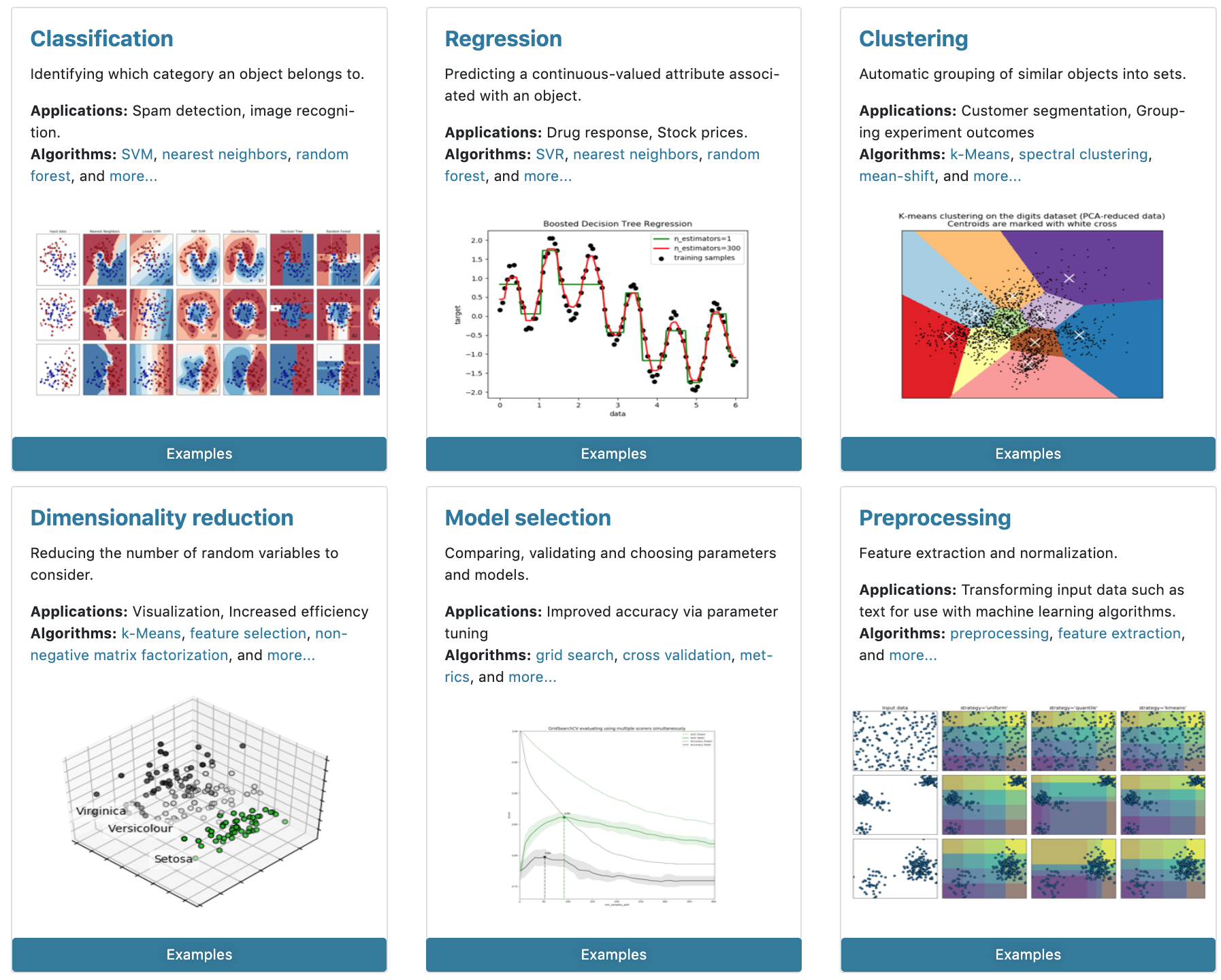
Scikit-learn Modules (Source: Scikit-learn Homepage)

A Brief History of Scikit-learn

Scikit-learn has come a long way from when it started back in 2007 as scikits.learn. Here’s a cool trivia for you – scikit-learn was a Google Summer of Code project by David Cournapeau!

This was taken over and rewritten by Fabian Pedregosa, Gael Varoquaux, Alexandre Gramfort and Vincent Michel, all from the French Institute for Research in Computer Science and Automation and its first public release took place in 2010.

Since then, it has added a lot of features and survived the test of time as the most popular open-source machine learning library across languages and frameworks. The below infographic, prepared by our team, illustrates a brief timeline of all the scikit-learn features along with their version number:

The above infographics show the release of features since its inception as a public library for implementing Machine Learning Algorithms from 2010 to 2019

Today, Scikit-learn is being used by organizations across the globe, including the likes of Spotify, JP Morgan, Booking.com, Evernote, and many more. You can find the complete list here with testimonials I believe this is just the tip of the iceberg when it comes to this library’s popularity as there will a lot of small and big companies using scikit-learn at some stage of prototyping models.

The latest version of scikit-learn, v0.22, has more than 20 active contributors today. v0.22 has added some excellent features to its arsenal that provide resolutions for some major existing pain points along with some fresh features which were available in other libraries but often caused package conflicts.

We will cover them in detail here and also dive into how to implement them in Python.

Scikit-Learn v0.22 Updates

Along with bug fixes and performance improvements, here are some new features that are included in scikit-learn’s latest version.

Stacking Classifier & Regressor

Stacking is one of the more advanced ensemble techniques made popular by machine learning competition winners at DataHack & Kaggle. Let’s first try to briefly understand how it works.

Stacking is an ensemble learning technique that uses predictions from multiple models (for example, decision tree, KNN or SVM) to build a new model.

This model is used for making predictions on the test set. Below is a step-wise explanation I’ve taken from this excellent article on ensemble learning for a simple stacked ensemble:

1. The train set is split into 10 parts:
   
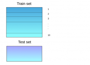
2. A base model (suppose a decision tree) is fitted on 9 parts and predictions are made for the 10th part. This is done for each part of the train set:
   
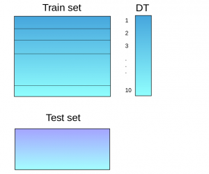
3. The base model (in this case, decision tree) is then fitted on the whole train dataset
4. Using this model, predictions are made on the test set:
   
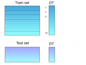
5. Steps 2 to 4 are repeated for another base model (say KNN) resulting in another set of predictions for the train set and test set:
   
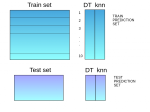
6. The predictions from the train set are used as features to build a new model:
   
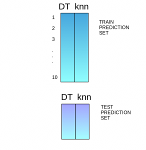
7. This model is used to make final predictions on the test prediction set

The mlxtend library provides an API to implement Stacking in Python. Now, sklearn, with its familiar API can do the same and it’s pretty intuitive as you will see in the demo below. You can either import StackingRegressor & StackingClassifier depending on your use case:

from sklearn.linear_model import LogisticRegression
from sklearn.ensemble import RandomForestClassifier
from sklearn.tree import DecisionTreeClassifier
from sklearn.ensemble import StackingClassifier
from sklearn.model_selection import train_test_split

X, y = load_iris(return_X_y=True)
estimators = [
    ('rf', RandomForestClassifier(n_estimators=10, random_state=42)),
    ('dt', DecisionTreeClassifier(random_state=42))
]
clf = StackingClassifier(estimators=estimators, final_estimator=LogisticRegression())

X_train, X_test, y_train, y_test = train_test_split(X, y, stratify=y, random_state=42)

clf.fit(X_train, y_train).score(X_test, y_test)

Permutation-Based Feature Importance

As the name suggests, this technique provides a way to assign importance to each feature by permuting each feature and capturing the drop in performance.

But what does permuting mean here? Let us understand this using an example.

Let’s say we are trying to predict house prices and have only 2 features to work with:

• LotArea – (Sq Feet area of the house)
• YrSold (Year when it was sold)

The test data has just 10 rows as shown below:

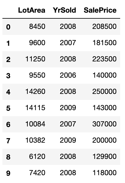
Next, we fit a simple decision tree model and get an R-Squared value of 0.78. We pick a feature, say LotArea, and shuffle it keeping all the other columns as they were:

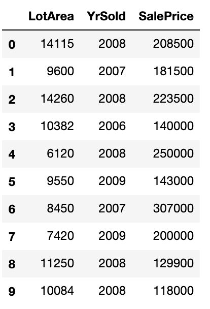
Next, we calculate the R-Squared once more and it comes out to be 0.74. We take the difference or ratio between the 2 (0.78/0.74 or 0.78-0.74), repeat the above steps, and take the average to represent the importance of the LotArea feature.

We can perform similar steps for all the other features to get the relative importance of each feature. Since we are using the test set here to evaluate the importance values, only the features that help the model generalize better will fare better.

Earlier, we had to implement this from scratch or import packages such as ELI5. Now, Sklearn has an inbuilt facility to do permutation-based feature importance. Let’s get into the code to see how we can visualize this:

from sklearn.ensemble import RandomForestClassifier
from sklearn.inspection import permutation_importance
from sklearn.datasets import make_classification
import matplotlib.pyplot as plt

# Use Sklearn make classification to create a dummy dataset with 3 important variables out of 7
X, y = make_classification(random_state=0, n_features=7, n_informative=3)
rf = RandomForestClassifier(random_state=0).fit(X, y)

result = permutation_importance(rf, X, y, 
                                n_repeats=10, # Number of times for which each feature must be shuffled
                                random_state=0, # random state fixing for reproducability
                                n_jobs=-1) # Parallel processing using all cores

fig, ax = plt.subplots()
sorted_idx = result.importances_mean.argsort()

ax.boxplot(result.importances[sorted_idx].T,
           vert=False, labels=range(X.shape[1]))

ax.set_title("Permutation Importance of each feature")
ax.set_ylabel("Features")

fig.tight_layout()
plt.show()

As you can see in the above box plot, there are 3 features that are relatively more important than the other 4. You can try this with any model, which makes it a model agnostic interpretability technique. You can read more about this machine learning interpretability concept here.

Multiclass Support for ROC-AUC

The ROC-AUC score for binary classification is super useful especially when it comes to imbalanced datasets. However, there was no support for Multi-Class classification till now and we had to manually code to do this. In order to use the ROC-AUC score for multi-class/multi-label classification, we would need to binarize the target first.

Currently, sklearn has support for two strategies in order to achieve this:

• One vs. One: Calculates the average of pairwise ROC AUC scores for each pair of classes (average=’macro’) <image>
• One vs. Rest: Calculate the average of ROC AUC scores for each class against all the others (average=’weighted’) <image>

from sklearn.datasets import load_iris 
from sklearn.ensemble import RandomForestClassifier

from sklearn.metrics import roc_auc_score
X, y = load_iris(return_X_y=True)

rf = RandomForestClassifier(random_state=44, max_depth=2)
rf.fit(X,y)

print(roc_auc_score(y, rf.predict_proba(X), multi_class='ovo'))

Also, there is a new plotting API that makes it super easy to plot and compare ROC-AUC curves from different machine learning models. Let’s see a quick demo:

from sklearn.model_selection import train_test_split
from sklearn.svm import SVC
from sklearn.metrics import plot_roc_curve
from sklearn.ensemble import RandomForestClassifier
from sklearn.datasets import make_classification
import matplotlib.pyplot as plt

X, y = make_classification(random_state=5)
X_train, X_test, y_train, y_test = train_test_split(X, y, random_state=42)

svc = SVC(random_state=42)
svc.fit(X_train, y_train)
rfc = RandomForestClassifier(random_state=42)
rfc.fit(X_train, y_train)

svc_disp = plot_roc_curve(svc, X_test, y_test)
rfc_disp = plot_roc_curve(rfc, X_test, y_test, ax=svc_disp.ax_)
rfc_disp.figure_.suptitle("ROC curve comparison")

plt.show()

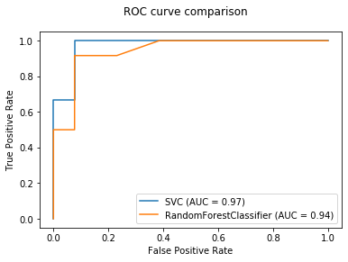
In the above figure, we have a comparison of two different machine learning models, namely Support Vector Classifier & Random Forest. Similarly, you can plot the AUC-ROC curve for more machine learning models and compare their performance.

kNN-Based Imputation

In kNN based imputation method, the missing values of an attribute are imputed using the attributes that are most similar to the attribute whose values are missing. The assumption behind using kNN for missing values is that a point value can be approximated by the values of the points that are closest to it, based on other variables.

The similarity of two attributes is determined using a distance function. Here are a few advantages of using kNN:

• • The k-nearest neighbor can predict both qualitative & quantitative attributes
  • Creation of predictive machine learning model for each attribute with missing data is not required
  • Correlation structure of the data is taken into consideration

Scikit-learn supports kNN-based imputation using the Euclidean distance method. Let’s see a quick demo:

import numpy as np
from sklearn.impute import KNNImputer
X = [[4, 6, np.nan], [3, 4, 3], [np.nan, 6, 5], [8, 8, 9]]
imputer = KNNImputer(n_neighbors=2)
print(imputer.fit_transform(X))

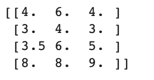
You can read about how kNN works in comprehensive detail here.

Tree Pruning

In basic terms, pruning is a technique we use to reduce the size of decision trees thereby avoiding overfitting. This also extends to other tree-based algorithms such as Random Forests and Gradient Boosting. These tree-based machine learning methods provide parameters such as min_samples_leaf and max_depth to prevent a tree from overfitting.

Pruning provides another option to control the size of a tree. XGBoost & LightGBM have pruning integrated into their implementation. However, a feature to manually prune trees has been long overdue in Scikit-learn (R already provides a similar facility as a part of the rpart package).

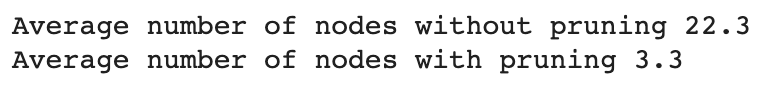
In its latest version, Scikit-learn provides this pruning functionality making it possible to control overfitting in most tree-based estimators once the trees are built. For details on how and why pruning is done, you can go through this excellent tutorial on tree-based methods by Sunil. Let’s look at a quick demo now:

from sklearn.ensemble import RandomForestClassifier 
from sklearn.datasets import make_classification

X, y = make_classification(random_state=0)

rf = RandomForestClassifier(random_state=0, ccp_alpha=0).fit(X, y)
print("Average number of nodes without pruning {:.1f}".format(
    np.mean([e.tree_.node_count for e in rf.estimators_])))

rf = RandomForestClassifier(random_state=0, ccp_alpha=0.1).fit(X, y)
print("Average number of nodes with pruning {:.1f}".format(
    np.mean([e.tree_.node_count for e in rf.estimators_])))

End Notes

The scikit-learn package is the ultimate go-to library for building machine learning models. It is the first machine learning-focused library all newcomers lean on to guide them through their initial learning process. And even as a veteran, I often find myself using it to quickly test out a hypothesis or solution I have in mind.

The latest release definitely has some significant upgrades as we just saw. It’s definitely worth exploring on your own and experimenting using the base I have provided in this article.

Have you tried out the latest version yet? Share your thoughts with the community in the comments section below.

Ankit Choudhary

IIT Bombay Graduate with a Masters and Bachelors in Electrical Engineering. I have previously worked as a lead decision scientist for Indian National Congress deploying statistical models (Segmentation, K-Nearest Neighbours) to help party leadership/Team make data-driven decisions. My interest lies in putting data in heart of business for data-driven decision making.