Overview
- Convolutional neural networks (CNNs) are all the rage in the deep learning and computer vision community
- How does this CNN architecture work? We’ll explore the math behind the building blocks of a convolutional neural network
- We will also build our own CNN from scratch using NumPy
Introduction
Convolutional neural network (CNN) – almost sounds like an amalgamation of biology, art and mathematics. In a way, that’s exactly what it is (and what this article will cover).
CNN-powered deep learning models are now ubiquitous and you’ll find them sprinkled into various computer vision applications across the globe. Just like XGBoost and other popular machine learning algorithms, convolutional neural networks came into the public consciousness through a hackathon (the ImageNet competition in 2012).
These neural networks have caught inspiration like fire since then, expanding into various research areas. Here are just a few popular computer vision applications where CNNs are used:
- Facial recognition systems
- Analyzing and parsing through documents
- Smart cities (traffic cameras, for example)
- Recommendation systems, among other use cases

But why does a convolutional neural network work so well? How does it perform better than the traditional ANNs (Artificial neural network)? Why do deep learning experts love it?
To answer these questions, we must understand how a CNN actually works under the hood. In this article, we will go through the mathematics behind a CNN model and we’ll then build our own CNN from scratch.
If you prefer a course format where we cover this content in stages, you can enrol in this free course: Convolutional Neural Networks from Scratch
Note: If you’re new to neural networks, I highly recommend checking out our popular free course:
Table of Contents
- Introduction to Neural Networks
- Forward Propagation
- Backward Propagation
- Convolutional Neural Network (CNN) Architecture
- Forward Propagation in CNNs
- Convolutional Layer
- Linear Transformation
- Non-linear Transformation
- Forward Propagation Summary
- Backward Propagation in CNNs
- Fully Connected Layer
- Convolution Layer
- CNN from Scratch using NumPy
Introduction to Neural Networks
Neural Networks are at the core of all deep learning algorithms. But before you deep dive into these algorithms, it’s important to have a good understanding of the concept of neural networks.
These neural networks try to mimic the human brain and its learning process. Like a brain takes the input, processes it and generates some output, so does the neural network.
These three actions – receiving input, processing information, generating output – are represented in the form of layers in a neural network – input, hidden and output. Below is a skeleton of what a neural network looks like:
These individual units in the layers are called neurons. The complete training process of a neural network involves two steps.
1. Forward Propagation
Images are fed into the input layer in the form of numbers. These numerical values denote the intensity of pixels in the image. The neurons in the hidden layers apply a few mathematical operations on these values (which we will discuss later in this article).
In order to perform these mathematical operations, there are certain parameter values that are randomly initialized. Post these mathematical operations at the hidden layer, the result is sent to the output layer which generates the final prediction.
2. Backward Propagation
Once the output is generated, the next step is to compare the output with the actual value. Based on the final output, and how close or far this is from the actual value (error), the values of the parameters are updated. The forward propagation process is repeated using the updated parameter values and new outputs are generated.
This is the base of any neural network algorithm. In this article, we will look at the forward and backward propagation steps for a convolutional neural network!
Convolutional Neural Network (CNN) Architecture
Consider this – you are asked to identify objects in two given images. How would you go about doing that? Typically, you would observe the image, try to identify different features, shapes and edges from the image. Based on the information you gather, you would say that the object is a dog or a car and so on.
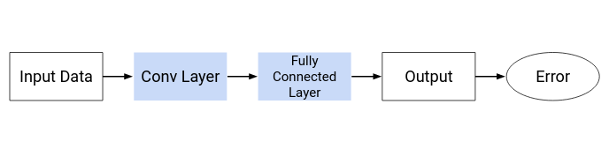
This is precisely what the hidden layers in a CNN do – find features in the image. The convolutional neural network can be broken down into two parts:
- The convolution layers: Extracts features from the input
- The fully connected (dense) layers: Uses data from convolution layer to generate output
As we discussed in the previous section, there are two important processes involved in the training of any neural network:
- Forward Propagation: Receive input data, process the information, and generate output
- Backward Propagation: Calculate error and update the parameters of the network
We will cover both of these one by one. Let us start with the forward propagation process.
Convolutional Neural Network (CNN): Forward Propagation
Convolution Layer
You know how we look at images and identify the object’s shape and edges? A convolutional neural network does this by comparing the pixel values.
Below is an image of the number 8 and the pixel values for this image. Take a look at the image closely. You would notice that there is a significant difference between the pixel values around the edges of the number. Hence, a simple way to identify the edges is to compare the neighboring pixel value.
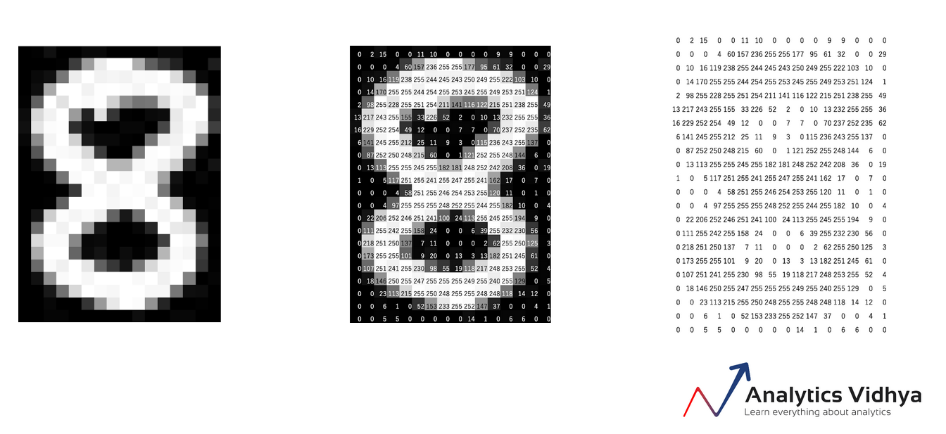
Do we need to traverse pixel by pixel and compare these values? No! To capture this information, the image is convolved with a filter (also known as a ‘kernel’).
Convolution is often represented mathematically with an asterisk * sign. If we have an input image represented as X and a filter represented with f, then the expression would be:
Z = X * f
Note: To learn how filters capture information about the edges, you can go through this article:
Let us understand the process of convolution using a simple example. Consider that we have an image of size 3 x 3 and a filter of size 2 x 2:
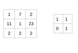
The filter goes through the patches of images, performs an element-wise multiplication, and the values are summed up:
(1x1 + 7x1 + 11x0 + 1x1) = 9
(7x1 + 2x1 + 1x0 + 23x1) = 32
(11x1 + 1x1 + 2x0 + 2x1) = 14
(1x1 + 23x1 + 2x0 + 2x1) = 26
Look at that closely – you’ll notice that the filter is considering a small portion of the image at a time. We can also imagine this as a single image broken down into smaller patches, each of which is convolved with the filter.
In the above example, we had an input of shape (3, 3) and a filter of shape (2, 2). Since the dimensions of image and filter are very small, it’s easy to interpret that the shape of the output matrix is (2, 2). But how would we find the shape of an output for more complex inputs or filter dimensions? There is a simple formula to do so:
Dimension of image = (n, n)
Dimension of filter = (f,f)

Dimension of output will be ((n-f+1) , (n-f+1))
You should have a good understanding of how a convolutional layer works at this point. Let us move to the next part of the CNN architecture.
Fully Connected Layer
So far, the convolution layer has extracted some valuable features from the data. These features are sent to the fully connected layer that generates the final results. The fully connected layer in a CNN is nothing but the traditional neural network!
The output from the convolution layer was a 2D matrix. Ideally, we would want each row to represent a single input image. In fact, the fully connected layer can only work with 1D data. Hence, the values generated from the previous operation are first converted into a 1D format.
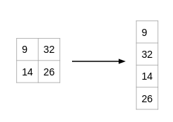
Once the data is converted into a 1D array, it is sent to the fully connected layer. All of these individual values are treated as separate features that represent the image. The fully connected layer performs two operations on the incoming data – a linear transformation and a non-linear transformation.
We first perform a linear transformation on this data. The equation for linear transformation is:
Z = WT.X + b
Here, X is the input, W is weight, and b (called bias) is a constant. Note that the W in this case will be a matrix of (randomly initialized) numbers. Can you guess what would be the size of this matrix?
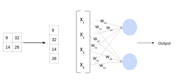
Considering the size of the matrix is (m, n) – m will be equal to the number of features or inputs for this layer. Since we have 4 features from the convolution layer, m here would be 4. The value of n will depend on the number of neurons in the layer. For instance, if we have two neurons, then the shape of weight matrix will be (4, 2):

Having defined the weight and bias matrix, let us put these in the equation for linear transformation:

Now, there is one final step in the forward propagation process – the non-linear transformations. Let us understand the concept of non-linear transformation and it’s role in the forward propagation process.
Non-Linear transformation
The linear transformation alone cannot capture complex relationships. Thus, we introduce an additional component in the network which adds non-linearity to the data. This new component in the architecture is called the activation function.
There are a number of activation functions that you can use – here is the complete list:
These activation functions are added at each layer in the neural network. The activation function to be used will depend on the type of problem you are solving.
We will be working on a binary classification problem and will use the Sigmoid activation function. Let’s quickly look at the mathematical expression for this:
f(x) = 1/(1+e^-x)
The range of a Sigmoid function is between 0 and 1. This means that for any input value, the result would always be in the range (0, 1). A Sigmoid function is majorly used for binary classification problems and we will use this for both convolution and fully-connected layers.
Let’s quickly summarize what we’ve covered so far.
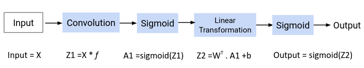
Forward Propagation Summary
Step 1: Load the input images in a variable (say X)
Step 2: Define (randomly initialize) a filter matrix. Images are convolved with the filter
Z1 = X * f
Step 3: Apply the Sigmoid activation function on the result
A = sigmoid(Z1)
Step 4: Define (randomly initialize) weight and bias matrix. Apply linear transformation on the values
Z2 = WT.A + b
Step 5: Apply the Sigmoid function on the data. This will be the final output
O = sigmoid(Z2)
Now the question is – how are the values in the filter decided? The CNN model treats these values as parameters, which are randomly initialized and learned during the training process. We will answer this in the next section.
Convolutional Neural Network (CNN): Backward Propagation
During the forward propagation process, we randomly initialized the weights, biases and filters. These values are treated as parameters from the convolutional neural network algorithm. In the backward propagation process, the model tries to update the parameters such that the overall predictions are more accurate.
For updating these parameters, we use the gradient descent technique. Let us understand the concept of gradient descent with a simple example.
Consider that following in the curve for our loss function where we have a parameter a:
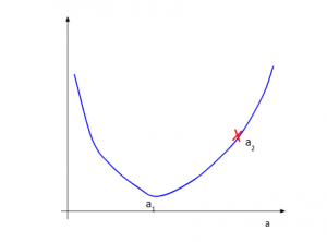
During the random initialization of the parameter, we get the value of a as a2. It is clear from the picture that the minimum value of loss is at a1 and not a2. The gradient descent technique tries to find this value of parameter (a) at which the loss is minimum.
We understand that we need to update the value a2 and bring it closer to a1. To decide the direction of movement, i.e. whether to increase or decrease the value of the parameter, we calculate the gradient or slope at the current point.
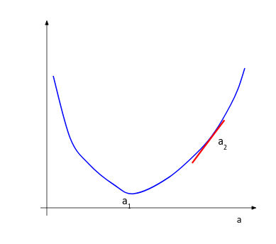
Based on the value of the gradient, we can determine the updated parameter values. When the slope is negative, the value of the parameter will be increased, and when the slope is positive, the value of the parameter should be decreased by a small amount.
Here is a generic equation for updating the parameter values:
new_parameter = old_parameter - (learning_rate * gradient_of_parameter)
The learning rate is a constant that controls the amount of change being made to the old value. The slope or the gradient determine the direction of the new values, that is, should the values be increased or decreased. So, we need to find the gradients, that is, change in error with respect to the parameters in order to update the parameter values.
If you want to read about the gradient descent technique in detail, you can go through the below article:
We know that we have three parameters in a CNN model – weights, biases and filters. Let us calculate the gradients for these parameters one by one.
Backward Propagation: Fully Connected Layer
As discussed previously, the fully connected layer has two parameters – weight matrix and bias matrix. Let us start by calculating the change in error with respect to weights – ∂E/∂W.
Since the error is not directly dependent on the weight matrix, we will use the concept of chain rule to find this value. The computation graph shown below will help us define ∂E/∂W:
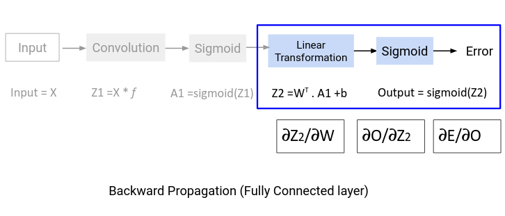
∂E/∂W = ∂E/∂O . ∂O/∂Z2. ∂z/∂W
We will find the values of these derivatives separately.
1. Change in error with respect to output
Suppose the actual values for the data are denoted as y’ and the predicted output is represented as O. Then the error would be given by this equation:
E = (y' - O)2/2
If we differentiate the error with respect to the output, we will get the following equation:
∂E/∂O = -(y'-O)
2. Change in output with respect to Z2 (linear transformation output)
To find the derivative of output O with respect to Z2, we must first define O in terms of Z2. If you look at the computation graph from the forward propagation section above, you would see that the output is simply the sigmoid of Z2. Thus, ∂O/∂Z2 is effectively the derivative of Sigmoid. Recall the equation for the Sigmoid function:
f(x) = 1/(1+e^-x)
The derivative of this function comes out to be:
f'(x) = (1+e-x)-1[1-(1+e-x)-1]
f'(x) = sigmoid(x)(1-sigmoid(x))
∂O/∂Z2 = (O)(1-O)
You can read about the complete derivation of the Sigmoid function here.
3. Change in Z2 with respect to W (Weights)
The value Z2 is the result of the linear transformation process. Here is the equation of Z2 in terms of weights:
Z2 = WT.A1 + b
On differentiating Z2 with respect to W, we will get the value A1 itself:
∂Z2/∂W = A1
Now that we have the individual derivations, we can use the chain rule to find the change in error with respect to weights:
∂E/∂W = ∂E/∂O . ∂O/∂Z2. ∂Z2/∂W

∂E/∂W = -(y'-o) . sigmoid'. A1
The shape of ∂E/∂W will be the same as the weight matrix W. We can update the values in the weight matrix using the following equation:
W_new = W_old - lr*∂E/∂W
Updating the bias matrix follows the same procedure. Try to solve that yourself and share the final equations in the comments section below!
Backward Propagation: Convolution Layer
For the convolution layer, we had the filter matrix as our parameter. During the forward propagation process, we randomly initialized the filter matrix. We will now update these values using the following equation:
new_parameter = old_parameter - (learning_rate * gradient_of_parameter)
To update the filter matrix, we need to find the gradient of the parameter – dE/df. Here is the computation graph for backward propagation:
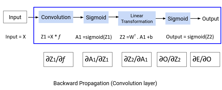
From the above graph we can define the derivative ∂E/∂f as:
∂E/∂f = ∂E/∂O.∂O/∂Z2.∂Z2/∂A1 .∂A1/∂Z1.∂Z1/∂f
We have already determined the values for ∂E/∂O and ∂O/∂Z2. Let us find the values for the remaining derivatives.
1. Change in Z2 with respect to A1
To find the value for ∂Z2/∂A1 , we need to have the equation for Z2 in terms of A1:
Z2 = WT.A1 + b
On differentiating the above equation with respect to A1, we get WT as the result:
∂Z2/∂A1 = WT
2. Change in A1 with respect to Z1
The next value that we need to determine is ∂A1/∂Z1. Have a look at the equation of A1
A1 = sigmoid(Z1)
This is simply the Sigmoid function. The derivative of Sigmoid would be:
∂A1/∂Z1 = (A1)(1-A1)
3. Change in Z1 with respect to filter f
Finally, we need the value for ∂Z1/∂f. Here’s the equation for Z1
Z1 = X * f
Differentiating Z with respect to X will simply give us X:
∂Z1/∂f = X
Now that we have all the required values, let’s find the overall change in error with respect to the filter:
∂E/∂f = ∂E/∂O.∂O/∂Z2.∂Z2/∂A1 .∂A1/∂Z1 * ∂Z1/∂f
Notice that in the equation above, the value (∂E/∂O.∂O/∂Z2.∂Z2/∂A1 .∂A1/∂Z) is convolved with ∂Z1/∂f instead of using a simple dot product. Why? The main reason is that during forward propagation, we perform a convolution operation for the images and filters.
This is repeated in the backward propagation process. Once we have the value for ∂E/∂f, we will use this value to update the original filter value:
f = f - lr*(∂E/∂f)
This completes the backpropagation section for convolutional neural networks. It’s now time to code!
CNN from Scratch using NumPy
Excited to get your hands dirty and design a convolutional neural network from scratch? The wait is over!
We will start by loading the required libraries and dataset. Here, we will be using the MNIST dataset which is present within the keras.datasets library.
For the purpose of this tutorial, we have selected only the first 200 images from the dataset. Here is the distribution of classes for the first 200 images:
1    26
9    23
7    21
4    21
3    21
0    21
2    20
6    19
8    15
5    13
dtype: int64
As you can see, we have ten classes here – 0 to 9. This is a multi-class classification problem. For now, we will start with building a simple CNN model for a binary classification problem:
0    109
1     91
dtype: int64
We will now initialize the filters for the convolution operation:
Let us quickly check the shape of the loaded images, target variable and the filter matrix:
X.shape, y.shape, f.shape
((28, 28, 200), (1, 200), (5, 5, 3))
We have 200 images of dimensions (28, 28) each. For each of these 200 images, we have one class specified and hence the shape of y is (1, 200). Finally, we defined 3 filters, each of dimensions (5, 5).
The next step is to prepare the data for the convolution operation. As we discussed in the forward propagation section, the image-filter convolution can be treated as a single image being divided into multiple patches:
For every single image in the data, we will create smaller patches of the same dimension as the filter matrix, which is (5, 5). Here is the code to perform this task:
(200, 576, 5, 5)
We have everything we need for the forward propagation process of the convolution layer. Moving on to the next section for forward propagation, we need to initialize the weight matrix for the fully connected layer. The size of the weight matrix will be (m, n) – where m is the number of features as input and n will be the number of neurons in the layer.
What would be the number of features? We know that we can determine the shape of the output image using this formula:
((n-f+1) , (n-f+1))
Since the fully connected layer only takes 1D input, we will flatten this matrix. This means the number of features or input values will be:
((n-f+1) x (n-f+1) x num_of_filter)
Let us initialize the weight matrix:
Finally, we will write the code for the activation function which we will be using for the convolution neural network architecture.
Now, we have already converted the original problem into a binary classification problem. Hence, we will be using Sigmoid as our activation function. We have already discussed the mathematical equation for Sigmoid and its derivative. Here is the python code for the same:
Great! We have all the elements we need for the forward propagation process. Let us put these code blocks together.
First, we perform the convolution operation on the patches created. After the convolution, the results are stored in the form of a list, which is converted into an array of dimension (200, 3, 576). Here
- 200 is the number of images
- 576 is the number of patches created, and
- 3 is the number of filters we used
After the convolution operation, we apply the Sigmoid activation function:
((200, 3, 576), (200, 3, 576))
After the convolution layer, we have the fully connected layer. We know that the fully connected layer will only have 1D inputs. So, we first flatten the results from the previous layer using the reshape function. Then, we apply the linear transformation and activation function on this data:
It’s time to start the code for backward propagation. Let’s define the individual derivatives for backward propagation of the fully connected layer. Here are the equations we need:
E = (y' - O)2/2
∂E/∂O = -(y'-O)
∂O/∂Z2 = (O)(1-O)
∂Z2/∂W = A1
Let us code this in Python:
We have the individual derivatives from the previous code block. We can now find the overall change in error w.r.t. weight using the chain rule. Finally, we will use this gradient value to update the original weight matrix:
W_new = W_old - lr*∂E/∂W
So far we have covered backpropagation for the fully connected layer. This covers updating the weight matrix. Next, we will look at the derivatives for backpropagation for the convolutional layer and update the filters:
∂E/∂f = ∂E/∂O.∂O/∂Z2.∂Z2/∂A1 .∂A1/∂Z1 * ∂Z1/∂f
∂E/∂O = -(y'-O)
∂O/∂Z2 = (O)(1-O)
∂Z2/∂A1 = WT
∂A1/∂Z1= A1(1-A1)
∂Z1/∂f = X
We will code the first four equations in Python and calculate the derivative using the np.dot function. Post that we need to perform a convolution operation using ∂Z1/∂f:
We now have the gradient value. Let us use it to update the error:
End Notes
Take a deep breath – that was a lot of learning in one tutorial! Convolutional neural networks can appear to be slightly complex when you’re starting out but once you get the hang of how they work, you’ll feel ultra confident in yourself.
I had a lot of fun writing about what goes on under the hood of these CNN models we see everywhere these days. We covered the mathematics behind these CNN models and learned how to implement them from scratch, using just the NumPy library.
I want you to explore other concepts related to CNN, such as the padding and pooling techniques. Implement them in the code as well and share your ideas in the comments section below.
You should also try your hand at the below hackathons to practice what you’ve learned:
backward propagationCNNconvolutional neural networkdeep learningfiltersforward propogationkernelNumPy
Aishwarya Singh
08 May, 2020
An avid reader and blogger who loves exploring the endless world of data science and artificial intelligence. Fascinated by the limitless applications of ML and AI; eager to learn and discover the depths of data science.


Very well written article, Aishwarya . Kudos !!
Glad you liked it Vipul!
Astounded. As someone just scratching at deep learning, this is the best "from nothing to a working example" I've seen so far, specially considering how the concepts do not skip any necessary parts and the code goes step-by-step. Really great job, and thanks for the article.
Thanks a lot Matheus!
very well written Aishwarya, congratulations, this is extremely useful and articulate
Thanks Avishek!
Amazing explanation. Great post. You have put an entire chapter in 1 page which is commendable. Thank you !!!
Hey it was amazing reading this! I have some doubt : 1) f=np.random.uniform(size=(3,5,5)) I didn't understand the concept of 3 here like the filter matrix is of size(5,5) so the filter matrix will be multiplied to the image matrix (28,28) with stripes (1,1) so whats the need of 3 matrix of size (5,5) thankyou once again for this amazing content
output_layer_input = (output_layer_input - np.average(output_layer_input))/np.std(output_layer_input) why we need to do the above step ? we can directly pass the dot product into sigmoid functions
Hi Himanshu, There are multiple ways to scale or normalize the values. Sigmoid is one, using this normalize is another. You can use any of these.
In wo = wo - lr*delta_error_fcp lr is not defined
Hi Anup, lr is the learning rate here. You can define it as lr = 0.01
first time, I got understand this very clearly. Thanks Aish.
Incredibly well done article. Congratulations to the author !!!
Very good explanation
Very good explanation of CNN underlying math architecture. Thanks!
thank you so much for the explanation. very very very..... helped me in understanding how filter weights are undated. thank you so much :-)