Key Difference between R-squared and Adjusted R-squared for Regression Analysis

Overview

• Understand the concept of R-squared and Adjusted R-Squared
• Get to know the key differences between R-Squared and Adjusted R-squared

Introduction

When I started my journey in Data Science, the first algorithm that I explored was Linear Regression. After understanding the concepts of Linear Regression and how the algorithm works, I was really excited to use it and make predictions on a problem statement. I am sure most of you would have done the same. But once we have predicted the values, what is next?

Then comes the tricky part. Once we have built our model, the next step was to evaluate its performance. Needless to say, the task of model evaluation is a pivotal one and highlights the shortcomings of our model. Choosing the most appropriate Evaluation Metric is a crucial task. And, I came across two important metrics: R-squared and Adjusted R-squared apart from MAE/ MSE/ RMSE. What is the difference between these two? Which one should I use?

R-squared and Adjusted R-squared are two such evaluation metrics that might seem confusing to any data science aspirant initially. Since they both are extremely important to evaluate regression problems, we are going to understand and compare them in-depth. They both have their pros and cons which we will be discussing in detail in this article.

Note: To understand R-Squared and Adjusted R-Squared, you must have a good understanding of Linear Regression. Please refer to our free course –

• Fundamentals of Regression Analysis

Residual Sum of Squares

To understand the concepts clearly, we are going to take up a simple regression problem. Here, we are trying to predict the ‘Marks Obtained’ based on the amount of ‘Time Spent Studying’. The time spent studying will be our independent variable and the marks achieved in the test is our dependent or target variable.

We can plot a simple regression graph to visualize this data.

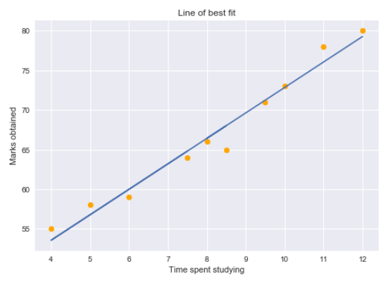
The yellow dots represent the data points and the blue line is our predicted regression line. As you can see, our regression model does not perfectly predict all the data points. So how do we evaluate the predictions from the regression line using the data? Well, we could start by determining the residual values for the data points.

Residual for a point in the data is the difference between the actual value and the value predicted by our linear regression model.

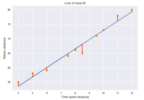
Residual plots tell us whether the regression model is the right fit for the data or not. It is actually an assumption of the regression model that there is no trend in residual plots. To study the assumptions of linear regression in detail, I suggest going through this great article!

Using the residual values, we can determine the sum of squares of the residuals also known as Residual sum of squares or RSS.

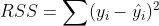
The lower the value of RSS, the better is the model predictions. Or we can say that – a regression line is a line of best fit if it minimizes the RSS value. But there is a flaw in this – RSS is a scale variant statistic. Since RSS is the sum of the squared difference between the actual and predicted value, the value depends on the scale of the target variable.

Example:

Consider your target variable is the revenue generated by selling a product. The residuals would depend on the scale of this target. If the revenue scale was taken in “Hundreds of Rupees” (i.e. target would be 1, 2, 3, etc.) then we might get an RSS of about 0.54 (hypothetically speaking).

But if the revenue target variable was taken in “Rupees” (i.e. target would be 100, 200, 300, etc.), then we might get a larger RSS as 5400. Even though the data does not change, the value of RSS varies according to the scale of the target. This makes it difficult to judge what might be a good RSS value.

So, can we come up with a better statistic that is scale-invariant? This is where R-squared comes into the picture.

Understanding R-squared statistic

R-squared statistic or coefficient of determination is a scale invariant statistic that gives the proportion of variation in target variable explained by the linear regression model.

This might seem a little complicated, so let me break this down here. In order to determine the proportion of target variation explained by the model, we need to first determine the following-

1. Total Sum of Squares

   Total variation in target variable is the sum of squares of the difference between the actual values and their mean.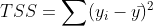

   

   TSS or Total sum of squares gives the total variation in Y. We can see that it is very similar to the variance of Y. While the variance is the average of the squared sums of difference between actual values and data points, TSS is the total of the squared sums.

   Now that we know the total variation in the target variable, how do we determine the proportion of this variation explained by our model? We go back to RSS.

2. Residual Sum of Squares

   As we discussed before, RSS gives us the total square of the distance of actual points from the regression line. But if we focus on a single residual, we can say that it is the distance that is not captured by the regression line. Therefore, RSS as a whole gives us the variation in the target variable that is not explained by our model.

3. Calculate R-Squared

Now, if TSS gives us the total variation in Y, and RSS gives us the variation in Y not explained by X, then TSS-RSS gives us the variation in Y that is explained by our model! We can simply divide this value by TSS to get the proportion of variation in Y that is explained by the model. And this our R-squared statistic!

R-squared = (TSS-RSS)/TSS

                    = Explained variation/ Total variation

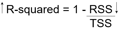
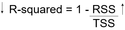
                    = 1 – Unexplained variation/ Total variation

So R-squared gives the degree of variability in the target variable that is explained by the model or the independent variables. If this value is 0.7, then it means that the independent variables explain 70% of the variation in the target variable.

R-squared value always lies between 0 and 1. A higher R-squared value indicates a higher amount of variability being explained by our model and vice-versa.

If we had a really low RSS value, it would mean that the regression line was very close to the actual points. This means the independent variables explain the majority of variation in the target variable. In such a case, we would have a really high R-squared value.

On the contrary, if we had a really high RSS value, it would mean that the regression line was far away from the actual points. Thus, independent variables fail to explain the majority of variation in the target variable. This would give us a really low R-squared value.

So, this explains why the R-squared value gives us the variation in the target variable given by the variation in independent variables.

Problems with R-squared statistic

The R-squared statistic isn’t perfect. In fact, it suffers from a major flaw. Its value never decreases no matter the number of variables we add to our regression model. That is, even if we are adding redundant variables to the data, the value of R-squared does not decrease. It either remains the same or increases with the addition of new independent variables. This clearly does not make sense because some of the independent variables might not be useful in determining the target variable. Adjusted R-squared deals with this issue.

What is Adjusted R-squared?

Adjusted R-squared is a statistical measure used to evaluate the goodness of fit of a regression model. It provides insights into how well the model explains the variability in the data.

Unlike the standard R-squared, which simply tells you the proportion of variance explained by the model, Adjusted R-squared takes into account the number of predictors (independent variables) in the model.

The advantage of Adjusted R-squared is that it penalizes the inclusion of unnecessary variables. This means that as you add more predictors to the model, the Adjusted R-squared value will only increase if the new variables significantly improve the model’s performance.

In summary, a higher Adjusted R-squared value indicates that more of the variation in the dependent variable is explained by the model, while also considering the model’s simplicity. It’s a valuable tool for model selection, helping you strike a balance between explanatory power and complexity.

Adjusted R-squared statistic

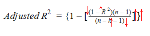
The Adjusted R-squared takes into account the number of independent variables used for predicting the target variable. In doing so, we can determine whether adding new variables to the model actually increases the model fit.

Let’s have a look at the formula for adjusted R-squared to better understand its working.

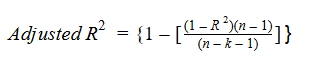
Here,

• n represents the number of data points in our dataset
• k represents the number of independent variables, and
• R represents the R-squared values determined by the model.

So, if R-squared does not increase significantly on the addition of a new independent variable, then the value of Adjusted R-squared will actually decrease.

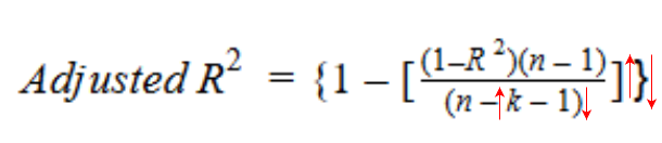
On the other hand, if on adding the new independent variable we see a significant increase in R-squared value, then the Adjusted R-squared value will also increase.

We can see the difference between R-squared and Adjusted R-squared values if we add a random independent variable to our model.

As you can see, adding a random independent variable did not help in explaining the variation in the target variable. Our R-squared value remains the same. Thus, giving us a false indication that this variable might be helpful in predicting the output. However, the Adjusted R-squared value decreased which indicated that this new variable is actually not capturing the trend in the target variable.

Clearly, it is better to use Adjusted R-squared when there are multiple variables in the regression model. This would allow us to compare models with differing numbers of independent variables.

Frequently Asked Questions

End Notes

In this article, we looked at what the R-squared statistic is and where does it falter. We also had a look at Adjusted R-squared.

Hopefully, this has given you a better understanding of things. You can now determine prudently which independent variables are helpful in predicting the output of your regression problem.

To know more about other evaluation metrics, I suggest going through the following great resources:

• 11 Important Model Evaluation Metrics for Machine Learning
• Evaluation Metrics for Machine Learning Models (free course)