How to Reduce Computational Constraints using Momentum Contrast V2(Moco-v2) in PyTorch

Introduction

The SimCLR paper explains how this framework benefits from larger models and larger batch sizes and can produce results comparable to those of supervised models if enough computing power is available. But these requirements make the framework quite computation-heavy. Wouldn’t it be wonderful if we could have the simplicity and power of this framework and have fewer compute requirements so that this can become accessible to everyone? Moco-v2 comes to the rescue.

Note: In a previous blog post, we implemented the SimCLR framework in PyTorch, on a simple dataset of 5 categories with a total of just 1250 training images.

Dataset

We will implement Moco-v2 in PyTorch on much bigger datasets this time and train our model on Google Colab. We will work with the Imagenette and Imagewoof datasets this time, made by Jeremy Howard from Fast.AI.

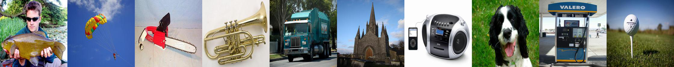
Some images from the Imagewoof dataset

A quick summary of these datasets (more info is here):

• Imagenette consists of 10 easily classified classes from Imagenet with a total of 9479 training and 3935 validation set images.
• Imagewoof is a dataset of 10 difficult classes from Imagenet — difficult because all classes are dog breeds. There’re a total of 9035 training, and 3939 validation set images.

Contrastive Learning — A Review

The way contrastive learning works in self-supervised learning is based on the idea that we want different outlooks of images from the same category to have similar representations. But since we don’t know which images belong to the same category, what is generally done is that representations of different outlooks of the same image are brought closer to each other. We call these different views taken pairwise as positive pairs.

But a constant representation fulfills this idea. So, additionally, we want different outlooks of images from different categories to have representations far from each other. But again, given the lack of information about the categories, instead representations of different outlooks of different images irrespective of the category are pushed away from each other. We call these different views taken pairwise as negative pairs.

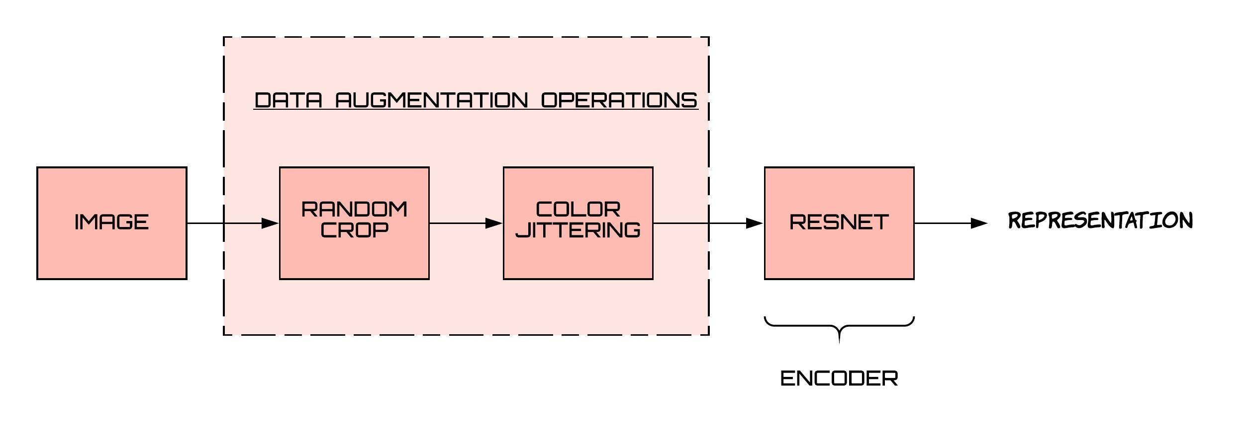
What’s an outlook of an image in this context? An outlook can be thought of as a way of looking at some part of the image in a modified way, it’s essentially a transformation of the image. Some transformations can work better than others, depending on the task at hand. SimCLR showed that applying random crop and then color jittering works quite well on a variety of tasks, including image classification. This essentially came from a grid search of choosing a pair of transformations from choices like rotate, crop, cut out, noise, blur, Sobel filtering, etc.

The mapping from the outlook to the representation space is done through a neural network, and typically, a resnet is used for this purpose. The following is the pipeline from images to representations-

How are negative pairs generated?

From the same image, we can get multiple representations because of random cropping. In this way, we can generate positive pairs. But how to generate negative pairs? Negative pairs are representations that come from different images. The SimCLR paper created these in the same batch. If a batch contains N images, then for each image, we get 2 representations, which accounts for a total of 2*N representations. For a particular representation x, there is one representation that forms a positive pair with x (the one that comes from the same image as x) and rest all (exactly 2*N – 2) form negative pairs with x.

The representations improve if we have a large number of negative samples at hand. But a large no. of negative samples can be accomplished in the case of SimCLR only if we have large batch sizes, which leads to higher computing power requirements. Momentum Contrast v2 (MoCo-v2) provides an alternate approach to generating negative samples. Let’s understand it in detail.

Dynamic Dictionaries

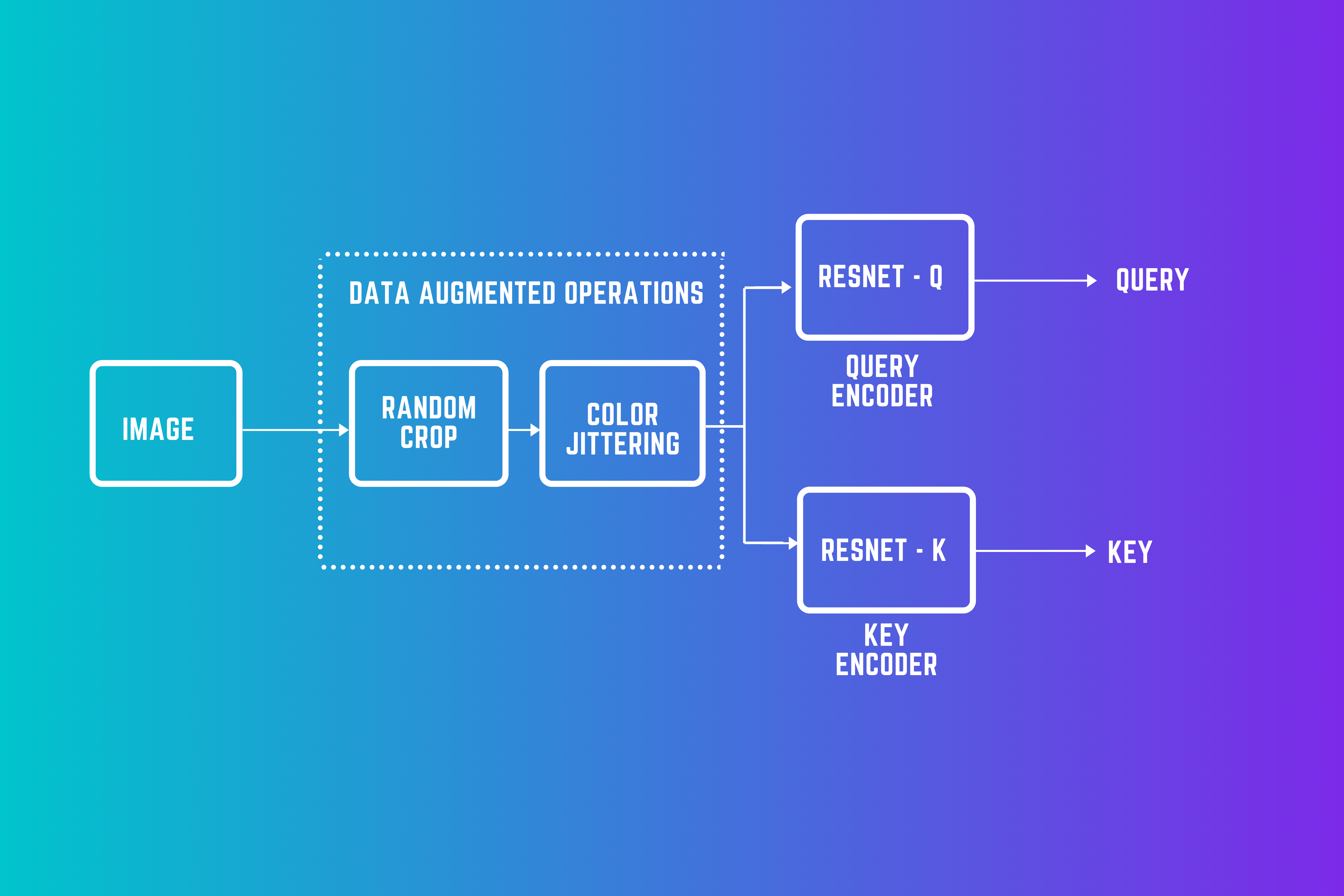
We can look at the contrastive learning approach in a slightly different way i.e., matching queries to keys. Instead of having a single encoder, we now have two encoders — one for query and another one for the key. Moreover, to have a large number of negative samples, we have a large dictionary of encoded keys.

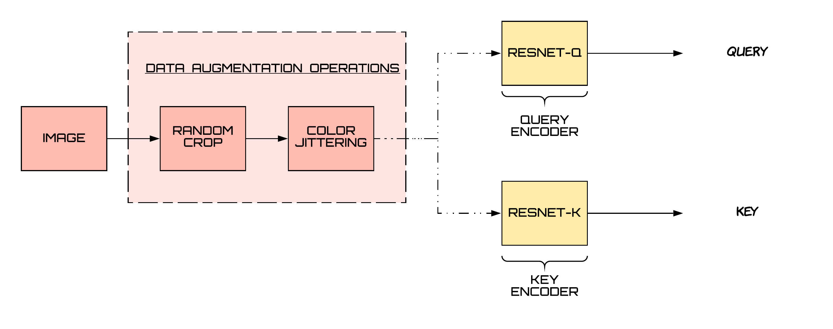
A positive pair in this context means that the query matches the key. They match if both the query and the key come from the same image. An encoded query should be similar to its matching key and dissimilar to others [1].

For negative pairs, we maintain a large dictionary which contains encoded keys from previous batches. They serve as negative samples to the query at hand. We maintain the dictionary in the form of a queue. The latest batch is enqueued and the oldest batch is dequeued. By changing the size of this queue, change the number of negative samples.

Challenges with this approach

• As the key encoder changes, the keys which are enqueued at later points of time can become inconsistent with the keys that were enqueued quite early. For the contrastive learning approach to work, all the keys that are compared to the queries must come from the same or similar encoders for the comparisons to be meaningful and consistent.
• Another challenge is that it’s not feasible to learn the key encoder parameters using backpropagation because that would require calculating gradients for all the samples in the queue (which would result in a large computational graph).

To address both of these issues, MoCo implements the key encoder as a momentum-based moving average of the query encoder [1]. It means that it updates the key encoder parameters in this way:

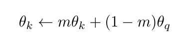
where m is kept quite close to 1 (e.g., a typical value is 0.999), which ensures that we obtain the encoded keys at different times from similar encoders.

The Loss Function — InfoNCE

We want a query to be close to all its positive and be far from all its negative samples. The InfoNCE loss function captures it. It stands for Information Noise Contrastive Estimation. InfoNCE loss function for a query q, for which the positive key is kᵣ is:

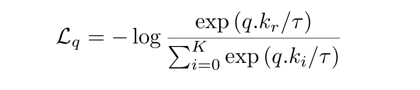
which we can rewrite to get this form:

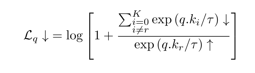
The following is the code for the loss function:

τ = 0.05

def loss_function(q, k, queue):

    # N is the batch size
    N = q.shape[0]
    
    # C is the dimensionality of the representations
    C = q.shape[1]

    # bmm stands for batch matrix multiplication
    # If mat1 is a b×n×m tensor, mat2 is a b×m×p tensor, 
    # then output will be a b×n×p tensor. 
    pos = torch.exp(torch.div(torch.bmm(q.view(N,1,C), k.view(N,C,1)).view(N, 1),τ))
    
    # performs matrix multiplication between query and queue tensors
    neg = torch.sum(torch.exp(torch.div(torch.mm(q.view(N,C), torch.t(queue)),τ)), dim=1)
   
    # sum is over positive as well as negative samples
    denominator = neg + pos

    return torch.mean(-torch.log(torch.div(pos,denominator)))

Let’s take another look at this loss function and compare it with the categorical cross-entropy loss function.

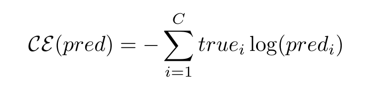
You can watch this video to understand cross-entropy better if you’re new to the topic. Also, note that we often convert the scores to probability values through a function like softmax.

We can think of the InfoNCE Loss function as the cross-entropy loss. The correct class for the data sample “q” is the rᵗʰ class, with the underlying classifier being softmax-based, which is trying to classify between K+1 classes.

The Info-NCE loss is also related to the mutual information between the encoded representations; more details on this are present in [4].

The MoCo-v2 Framework

Now, let’s put all the things together and see how the entire Moco-v2 Algorithm looks.

Step1:

We have to get the query and key encoders. Initially, the key encoder has the same parameters as that of the query encoder. They are copies of each other. As the training progresses, the key encoder would become a moving average (a slowly progressing at that one) of the query encoder.

We use the Resnet-18 architecture for our implementation because of computational power limitations. On top of the usual resnet architecture, we add some dense layers, to get the dimensionality of the representations down to 25. Some of these layers will act as a projection head later on, just like what we did in SimCLR.

# defining our deep learning architecture
resnetq = resnet18(pretrained=False)

classifier = nn.Sequential(OrderedDict([
    ('fc1', nn.Linear(resnetq.fc.in_features, 100)),
    ('added_relu1', nn.ReLU(inplace=True)),
    ('fc2', nn.Linear(100, 50)),
    ('added_relu2', nn.ReLU(inplace=True)),
    ('fc3', nn.Linear(50, 25))
]))

resnetq.fc = classifier
resnetk = copy.deepcopy(resnetq)

# moving the resnet architecture to device
resnetq.to(device)
resnetk.to(device)

Step2:

Now, as we have got our encoders and assuming that we have other crucial data structures set up, it’s time to start the training loop and understand the pipeline.

This step is about getting encoded queries and keys from the training batch. We normalize the representations by their L2-norm.

Just a convention alert, the code in all the subsequent steps will be inside both loops for batches and epochs. We also detach the tensor “k” from its grad, because we won’t be needing the key encoder part of our computational graph, as the momentum update equation would update our key encoder.

# zero out grads
optimizer.zero_grad()

# retrieve xq and xk the two image batches
xq = sample_batched['image1']
xk = sample_batched['image2']

# move them to the device
xq = xq.to(device)
xk = xk.to(device)

# get their outputs
q = resnetq(xq)
k = resnetk(xk)
k = k.detach()

# normalize the ouptuts, make them unit vectors
q = torch.div(q,torch.norm(q,dim=1).reshape(-1,1))
k = torch.div(k,torch.norm(k,dim=1).reshape(-1,1))

Step3:

Now, we pass our queries, keys, and the queue to our previously defined loss function and store the value in a list. Then, as usual, we call the backward function on our loss value and run the optimizer.

# get loss value
loss = loss_function(q, k, queue)

# put that loss value in the epoch losses list
epoch_losses_train.append(loss.cpu().data.item())

# perform backprop on loss value to get gradient values
loss.backward()

# run the optimizer
optimizer.step()

Step4:

We enqueue the latest batch in our queue. If our queue size gets larger than the maximum queue size that we defined (in K), then we dequeue the oldest batch from it. Enqueue operation can be done by using torch.cat and dequeue by simply index slicing the tensor.

# update the queue
queue = torch.cat((queue, k), 0) 

# dequeue if the queue gets larger than the max queue size - denoted by K
# batch size is 256, can be replaced by a variable
if queue.shape[0] > K:
    queue = queue[256:,:]

Step5:

Now we come to the final step of our training loop, which is to update the key encoder. We do this using the following for loop.

# update resnetk
for θ_k, θ_q in zip(resnetk.parameters(), resnetq.parameters()):
    θ_k.data.copy_(momentum*θ_k.data + θ_q.data*(1.0 - momentum))

Some Training Details

Training resnet-18 models took close to 18 hours of GPU time for each of the Imagenette and Imagewoof datasets. We used Google Colab’s GPU (16GB) for this purpose. We used a batch size of 256, a tau value of 0.05, a learning rate of 0.001, which we decreased eventually to 1e-5, and a weight decay of 1e-6. Our queue size was 8192 and the momentum value for the key encoder was 0.999.

Results

The top 3 layers (treating relu as a layer) defined our projection head, which we removed for the downstream task of image classification. On top of the remaining network, we trained a linear classifier.

We got an accuracy of 64.2% for Imagenette while using 10% of the labeled training data, using MoCo-v2. In comparison, using state of the art methods for supervised learning on it, close to 95% accuracy has been achieved.

And for Imagewoof, we got 38.6% accuracy for 10% labeled data. Contrastive learning on this dataset performed below our expectations. We suspect it is because firstly, the dataset is pretty tough since all classes are of dog species. Secondly, we think that color is an essential distinguishing feature of these classes. Applying color jittering may have resulted in multiple images from different classes to have representations intermingled with each other. In comparison, supervised methods have achieved close to 90% accuracy on it.

Design changes that can bridge the gap between self-supervised and supervised models:

1. Using bigger and wider models.
2. By using larger batch and dictionary sizes.
3. Using more data, if one can. Bringing in all the unlabeled data as well.
4. Training large models on large amounts of data and then distilling them.

Some useful links:

• Google Colab’s Notebook link
• Imagewoof Results Github Repo
• Imagenette Results Github Repo
• Imagewoof Dataset link
• Imagenette Dataset link

References

1. Momentum Contrast for Unsupervised Visual Representation Learning, Kaiming He, Haoqi Fan, Yuxin Wu, Saining Xie, and Ross Girshick
2. Improved Baselines with Momentum Contrastive Learning, Xinlei Chen, Haoqi Fan, Ross Girshick, and Kaiming He
3. A simple framework for contrastive learning of visual representations, Ting Chen, Simon Kornblith, Mohammad Norouzi, and Geoffrey E. Hinton.
4. Representation Learning with Contrastive Predictive Coding, Aaron van den Oord, Yazhe Li, and Oriol Vinyals

About the Author