Overview
- DBSCAN clustering is an underrated yet super useful clustering algorithm for unsupervised learning problems
- Learn how DBSCAN clustering works, why you should learn it, and how to implement DBSCAN clustering in Python
Introduction
Mastering unsupervised learning opens up a broad range of avenues for a data scientist. There is so much scope in the vast expanse of unsupervised learning and yet a lot of beginners in machine learning tend to shy away from it. In fact, I’m sure most newcomers will stick to basic clustering algorithms like K-Means clustering and hierarchical clustering.
While there’s nothing wrong with that approach, it does limit what you can do when faced with clustering projects. And why limit yourself when you can expand your learning, knowledge, and skillset by learning the powerful DBSCAN clustering algorithm?
Clustering is an essential technique in machine learning and is used widely across domains and industries (think about Uber’s route optimization, Amazon’s recommendation system, Netflix’s customer segmentation, and so on). This article is for anyone who wants to add an invaluable algorithm to their budding machine learning skillset – DBSCAN clustering!
Here, we’ll learn about the popular and powerful DBSCAN clustering algorithm and how you can implement it in Python. Also, you will get understanding of DBSCAN Algorithm , dbscanner what they are how they implemented so you will get a clear understanding of it .There’s a lot to unpack so let’s get rolling!
If you’re new to machine learning and unsupervised learning, check out this popular resource:
Table of contents
Why do we need DBSCAN Clustering?
This is a pertinent question. We already have basic clustering algorithms, so why should you spend your time and energy learning about yet another clustering method? It’s a fair question so let me answer that before I talk about what DBSCAN clustering is.
First, let’s clear up the role of clustering.
Clustering is an unsupervised learning technique where we try to group the data points based on specific characteristics. There are various clustering algorithms with K-Means and Hierarchical being the most used ones. Some of the use cases of clustering algorithms include:
- Document Clustering
- Recommendation Engine
- Image Segmentation
- Market Segmentation
- Search Result Grouping
- and Anomaly Detection.
All these problems use the concept of clustering to reach their end goal. Therefore, it is crucial to understand the concept of clustering. But here’s the issue with these two clustering algorithms.
K-Means and Hierarchical Clustering both fail in creating clusters of arbitrary shapes. They are not able to form clusters based on varying densities. That’s why we need DBSCAN clustering.
Let’s try to understand it with an example. Here we have data points densely present in the form of concentric circles:
We can see three different dense clusters in the form of concentric circles with some noise here. Now, let’s run K-Means and Hierarchical clustering algorithms and see how they cluster these data points.
You might be wondering why there are four colors in the graph? As I said earlier, this data contains noise too, therefore, I have taken noise as a different cluster which is represented by the purple color. Sadly, both of them failed to cluster the data points. Also, they were not able to properly detect the noise present in the dataset. Now, let’s take a look at the results from DBSCAN clustering.
Awesome! DBSCAN is not just able to cluster the data points correctly, but it also perfectly detects noise in the dataset.
What parameters required DBSCAN Algorithm?
The DBSCAN algorithm relies on two main parameters to identify clusters in your data:
- eps (ε): This parameter defines the radius of a neighborhood around a data point. Points within this distance are considered neighbors of the central point.
- minPts: This parameter represents the minimum number of points required within the ε-neighborhood of a point to classify it as a core point. A core point is considered to be dense enough to be part of a cluster.
These parameters work together to identify high-density regions in your data. Points with enough neighbors within the specified distance (core points) are grouped together as clusters, while points with insufficient neighbors are classified as noise.pen_sparktunesharemore_vert
What Exactly is DBSCAN Clustering?
DBSCAN stands for Density-Based Spatial Clustering of Applications with Noise.

It was proposed by Martin Ester et al. in 1996. DBSCAN is a density-based clustering algorithm that works on the assumption that clusters are dense regions in space separated by regions of lower density.
It groups ‘densely grouped’ data points into a single cluster. It can identify clusters in large spatial datasets by looking at the local density of the data points. The most exciting feature of DBSCAN clustering is that it is robust to outliers. It also does not require the number of clusters to be told beforehand, unlike K-Means, where we have to specify the number of centroids.
DBSCAN requires only two parameters: epsilon and minPoints. Epsilon is the radius of the circle to be created around each data point to check the density and minPoints is the minimum number of data points required inside that circle for that data point to be classified as a Core point.
In higher dimensions the circle becomes hypersphere, epsilon becomes the radius of that hypersphere, and minPoints is the minimum number of data points required inside that hypersphere.
Sounds confusing? Let’s understand it with the help of an example.
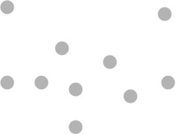
Here, we have some data points represented by grey color. Let’s see how DBSCAN clusters these data points.
DBSCAN creates a circle of epsilon radius around every data point and classifies them into Core point, Border point, and Noise. A data point is a Core point if the circle around it contains at least ‘minPoints’ number of points. If the number of points is less than minPoints, then it is classified as Border Point, and if there are no other data points around any data point within epsilon radius, then it treated as Noise.
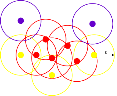
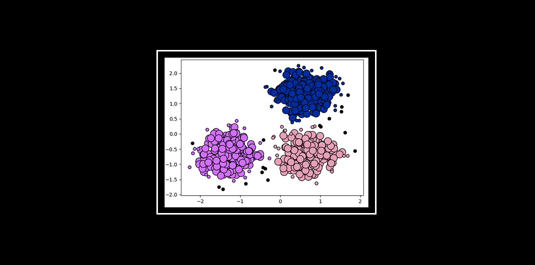
The above figure shows us a cluster created by DBCAN with minPoints = 3. Here, we draw a circle of equal radius epsilon around every data point. These two parameters help in creating spatial clusters.
All the data points with at least 3 points in the circle including itself are considered as Core points represented by red color. All the data points with less than 3 but greater than 1 point in the circle including itself are considered as Border points. They are represented by yellow color. Finally, data points with no point other than itself present inside the circle are considered as Noise represented by the purple color.
For locating data points in space, DBSCAN uses Euclidean distance, although other methods can also be used (like great circle distance for geographical data). It also needs to scan through the entire dataset once, whereas in other algorithms we have to do it multiple times.
Reachability and Connectivity
These are the two concepts that you need to understand before moving further. Reachability states if a data point can be accessed from another data point directly or indirectly, whereas Connectivity states whether two data points belong to the same cluster or not. In terms of reachability and connectivity, two points in DBSCAN can be referred to as:
- Directly Density-Reachable
- Density-Reachable
- Density-Connected
Let’s understand what they are.
A point X is directly density-reachable from point Y w.r.t epsilon, minPoints if,
- X belongs to the neighborhood of Y, i.e, dist(X, Y) <= epsilon
- Y is a core point
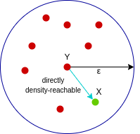
Here, X is directly density-reachable from Y, but vice versa is not valid.
A point X is density-reachable from point Y w.r.t epsilon, minPoints if there is a chain of points p1, p2, p3, …, pn and p1=X and pn=Y such that pi+1 is directly density-reachable from pi.
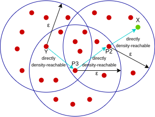
Here, X is density-reachable from Y with X being directly density-reachable from P2, P2 from P3, and P3 from Y. But, the inverse of this is not valid.
A point X is density-connected from point Y w.r.t epsilon and minPoints if there exists a point O such that both X and Y are density-reachable from O w.r.t to epsilon and minPoints.
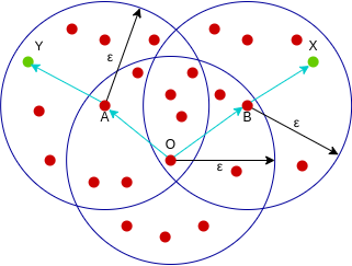
Here, both X and Y are density-reachable from O, therefore, we can say that X is density-connected from Y.
Parameter Selection in DBSCAN Clustering
DBSCAN is very sensitive to the values of epsilon and minPoints. Therefore, it is very important to understand how to select the values of epsilon and minPoints. A slight variation in these values can significantly change the results produced by the DBSCAN algorithm.
The value of minPoints should be at least one greater than the number of dimensions of the dataset, i.e.,
minPoints>=Dimensions+1.
It does not make sense to take minPoints as 1 because it will result in each point being a separate cluster. Therefore, it must be at least 3. Generally, it is twice the dimensions. But domain knowledge also decides its value.
The value of epsilon can be decided from the K-distance graph. The point of maximum curvature (elbow) in this graph tells us about the value of epsilon. If the value of epsilon chosen is too small then a higher number of clusters will be created, and more data points will be taken as noise. Whereas, if chosen too big then various small clusters will merge into a big cluster, and we will lose details.
Implementing DBSCAN Clustering in Python
Now, it’s implementation time! In this section, we’ll apply DBSCAN clustering on a dataset and compare its result with K-Means and Hierarchical Clustering.
Step 1-
Let’s start by importing the necessary libraries.
Python Code:
Step 2-
Here, I am creating a dataset with only two features so that we can visualize it easily. For creating the dataset I have created a function PointsInCircum which takes the radius and number of data points as arguments and returns an array of data points which when plotted forms a circle. We do this with the help of sin and cosine curves.
np.random.seed(42)

# Function for creating datapoints in the form of a circle
def PointsInCircum(r,n=100):
    return [(math.cos(2*math.pi/n*x)*r+np.random.normal(-30,30),math.sin(2*math.pi/n*x)*r+np.random.normal(-30,30)) for x in range(1,n+1)]
Step 3-
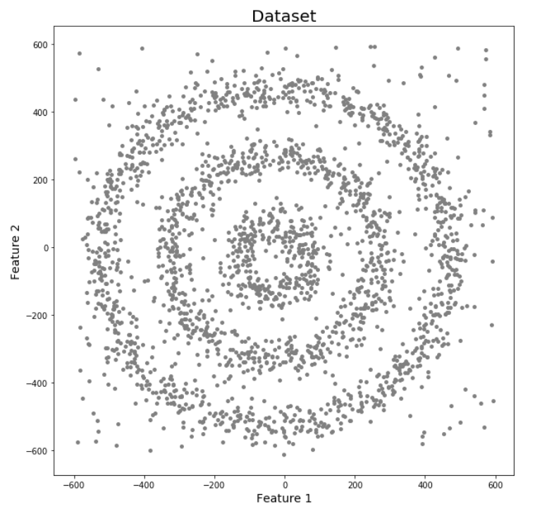
One circle won’t be sufficient to see the clustering ability of DBSCAN. Therefore, I have created three concentric circles of different radii. Also, I will add noise to this data so that we can see how different types of clustering algorithms deals with noise.
# Creating data points in the form of a circle
df=pd.DataFrame(PointsInCircum(500,1000))
df=df.append(PointsInCircum(300,700))
df=df.append(PointsInCircum(100,300))

# Adding noise to the dataset
df=df.append([(np.random.randint(-600,600),np.random.randint(-600,600)) for i in range(300)])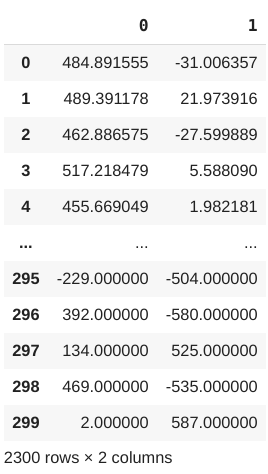
Step 4-
Let’s plot these data points and see how they look in the feature space. Here, I use the scatter plot for plotting these data points. Use the following syntax:
plt.figure(figsize=(10,10))
plt.scatter(df[0],df[1],s=15,color='grey')
plt.title('Dataset',fontsize=20)
plt.xlabel('Feature 1',fontsize=14)
plt.ylabel('Feature 2',fontsize=14)
plt.show()
Perfect! It’s excellent for clustering a problem.
If you want to know more about visualization in Python you can read the following articles:
- A Beginner’s Guide to matplotlib for Data Visualization and Exploration in Python
- Become a Data Visualization Whiz with this Comprehensive Guide to Seaborn in Python
- How to Create Beautiful, Interactive data visualizations using Plotly in R and Python?
K-Means vs. Hierarchical vs. DBSCAN Clustering
1. K-Means
We’ll first start with K-Means because it is the easiest clustering algorithm
from sklearn.cluster import KMeans
k_means=KMeans(n_clusters=4,random_state=42)
k_means.fit(df[[0,1]])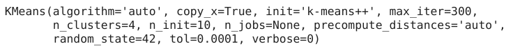
It’s time to see the results. Use labels_ to retrieve the labels. I have added these labels to the dataset in the new column so that data management can become easier. But don’t worry – I will only use two columns of the dataset for fitting other algorithms.
df['KMeans_labels']=k_means.labels_

# Plotting resulting clusters
colors=['purple','red','blue','green']
plt.figure(figsize=(10,10))
plt.scatter(df[0],df[1],c=df['KMeans_labels'],cmap=matplotlib.colors.ListedColormap(colors),s=15)
plt.title('K-Means Clustering',fontsize=20)
plt.xlabel('Feature 1',fontsize=14)
plt.ylabel('Feature 2',fontsize=14)
plt.show()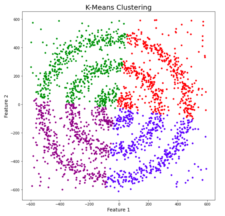
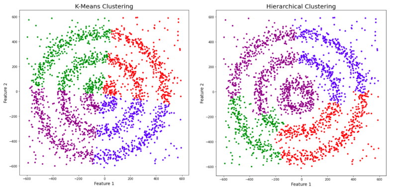
Here, K-means failed to cluster the data points into four clusters. Also, it didn’t work well with noise. Therefore, it is time to try another popular clustering algorithm, i.e., Hierarchical Clustering.
2. Hierarchical Clustering
For this article, I am performing Agglomerative Clustering but there is also another type of hierarchical clustering algorithm known as Divisive Clustering. Use the following syntax:
from sklearn.cluster import AgglomerativeClustering
model = AgglomerativeClustering(n_clusters=4, affinity='euclidean')
model.fit(df[[0,1]])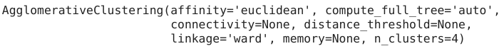
Here, I am taking labels from the Agglomerative Clustering model and plotting the results using a scatter plot. It is similar to what I did with KMeans.
df['HR_labels']=model.labels_

# Plotting resulting clusters
plt.figure(figsize=(10,10))
plt.scatter(df[0],df[1],c=df['HR_labels'],cmap=matplotlib.colors.ListedColormap(colors),s=15)
plt.title('Hierarchical Clustering',fontsize=20)
plt.xlabel('Feature 1',fontsize=14)
plt.ylabel('Feature 2',fontsize=14)
plt.show()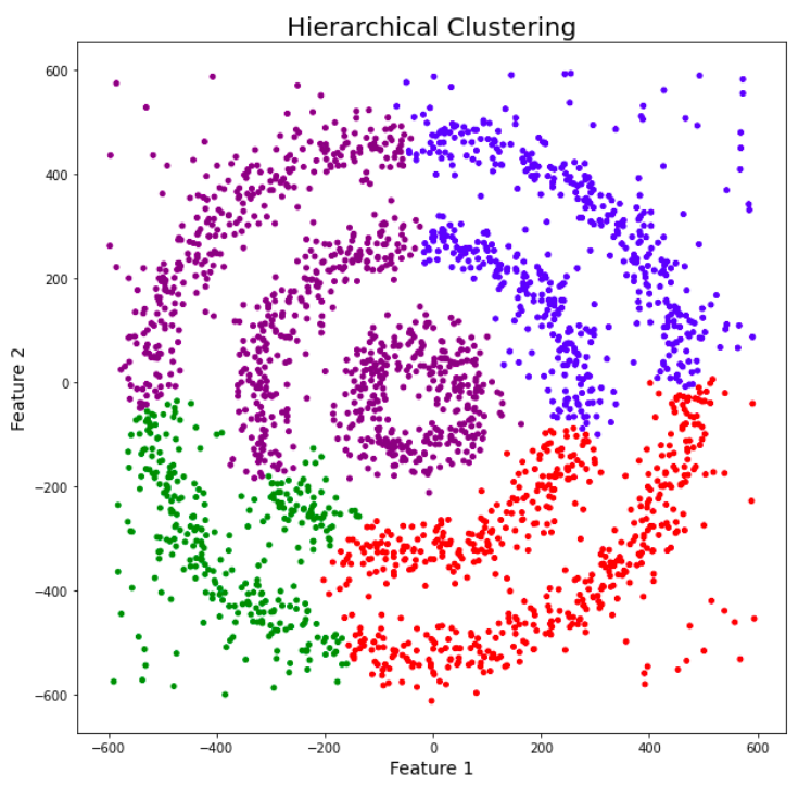
Sadly, the hierarchical clustering algorithm also failed to cluster the data points properly.
3. DBSCAN Clustering
Now, it’s time to implement DBSCAN and see its power. Import DBSCAN from sklearn.cluster. Let’s first run DBSCAN without any parameter optimization and see the results.
from sklearn.cluster import DBSCAN
dbscan=DBSCAN()
dbscan.fit(df[[0,1]])
Here, epsilon is 0.5, and min_samples or minPoints is 5. Let’s visualize the results from this model:df[‘DBSCAN_labels’]=dbscan.labels_
# Plotting resulting clusters
plt.figure(figsize=(10,10)) plt.scatter(df[0],df[1],c=df['DBSCAN_labels'],cmap=matplotlib.colors.ListedColormap(colors),s=15) plt.title('DBSCAN Clustering',fontsize=20)
plt.xlabel('Feature 1',fontsize=14)
plt.ylabel('Feature 2',fontsize=14)
plt.show()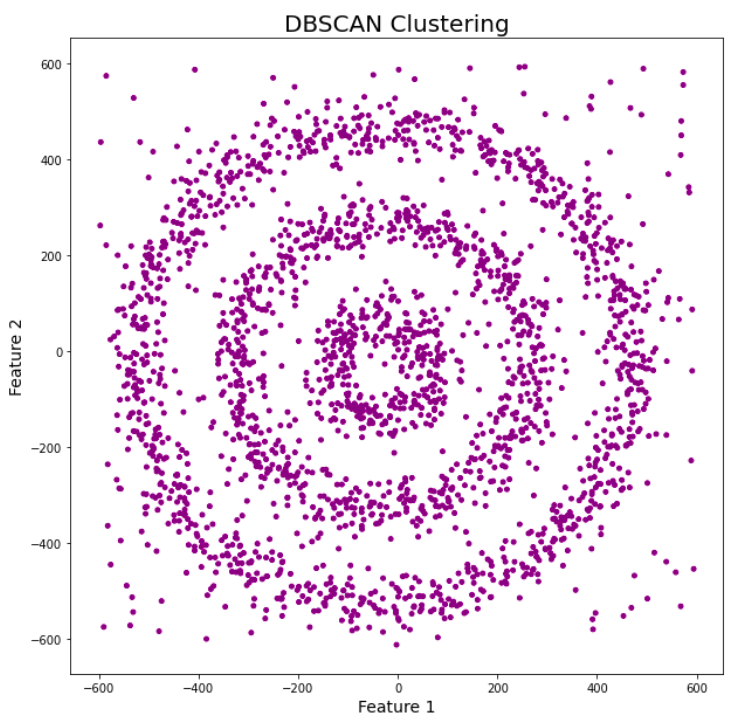
Interesting! All the data points are now of purple color which means they are treated as noise. It is because the value of epsilon is very small and we didn’t optimize parameters. Therefore, we need to find the value of epsilon and minPoints and then train our model again.
For epsilon, I am using the K-distance graph. For plotting a K-distance Graph, we need the distance between a point and its nearest data point for all data points in the dataset. We obtain this using NearestNeighbors from sklearn.neighbors.
from sklearn.neighbors import NearestNeighbors
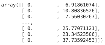
neigh = NearestNeighbors(n_neighbors=2)
nbrs = neigh.fit(df[[0,1]])
distances, indices = nbrs.kneighbors(df[[0,1]])The distance variable contains an array of distances between a data point and its nearest data point for all data points in the dataset.
Let’s plot our K-distance graph and find the value of epsilon. Use the following syntax:
# Plotting K-distance Graph
distances = np.sort(distances, axis=0)
distances = distances[:,1]
plt.figure(figsize=(20,10))
plt.plot(distances)
plt.title('K-distance Graph',fontsize=20)
plt.xlabel('Data Points sorted by distance',fontsize=14)
plt.ylabel('Epsilon',fontsize=14)
plt.show()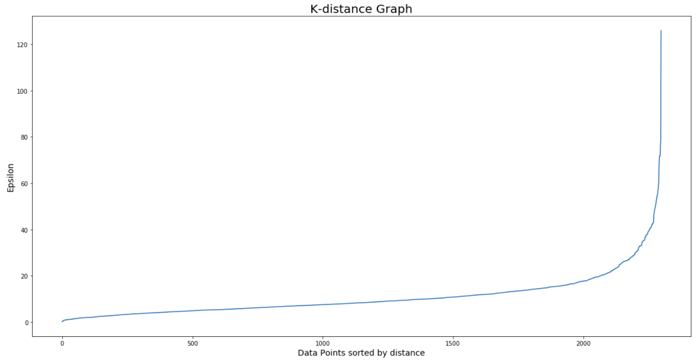
The optimum value of epsilon is at the point of maximum curvature in the K-Distance Graph, which is 30 in this case. Now, it’s time to find the value of minPoints. The value of minPoints also depends on domain knowledge. This time I am taking minPoints as 6:
from sklearn.cluster import DBSCAN
dbscan_opt=DBSCAN(eps=30,min_samples=6)
dbscan_opt.fit(df[[0,1]])
df['DBSCAN_opt_labels']=dbscan_opt.labels_
df['DBSCAN_opt_labels'].value_counts()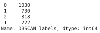
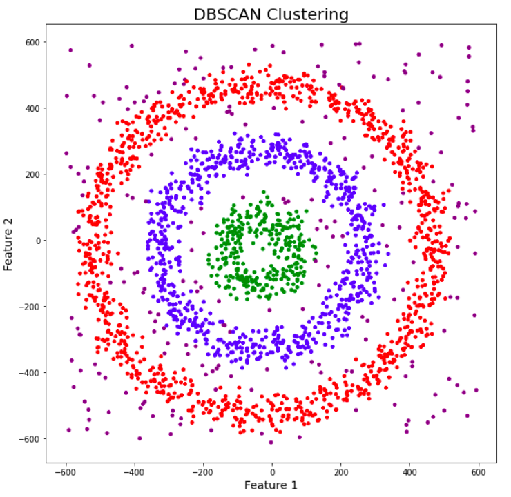
The most amazing thing about DBSCAN is that it separates noise from the dataset pretty well. Here, 0, 1 and 2 are the three different clusters, and -1 is the noise. Let’s plot the results and see what we get.
# Plotting the resulting clusters
plt.figure(figsize=(10,10))
plt.scatter(df[0],df[1],c=df['DBSCAN_opt_labels'],cmap=matplotlib.colors.ListedColormap(colors),s=15)
plt.title('DBSCAN Clustering',fontsize=20)
plt.xlabel('Feature 1',fontsize=14)
plt.ylabel('Feature 2',fontsize=14)
plt.show()
DBSCAN amazingly clustered the data points into three clusters, and it also detected noise in the dataset represented by the purple color.
One thing important to note here is that, though DBSCAN creates clusters based on varying densities, it struggles with clusters of similar densities. Also, as the dimension of data increases, it becomes difficult for DBSCAN to create clusters and it falls prey to the Curse of Dimensionality.
Conclusion
So in this article, I explained the DBSCAN clustering algorithm in-depth and also showcased how it is useful in comparison with other clustering algorithms. Also, note that there also exists a much better and recent version of this algorithm known as HDBSCAN which uses Hierarchical Clustering combined with regular DBSCAN. It is much faster and accurate than DBSCAN.Hope you like the article and get information about the dbscanner and dbscan algorithm . We cover all parts and information regarding about the dbscan clustering.
Frequently Asked Questions
Q1. What is DBSCAN used for?
A. DBSCAN (Density-Based Spatial Clustering of Applications with Noise) is a popular clustering algorithm used for data analysis and pattern recognition. It groups data points based on their density, identifying clusters of high-density regions and classifying outliers as noise. DBSCAN is effective in discovering arbitrary-shaped clusters in data and is widely used in data mining, spatial data analysis, and machine learning applications.
Q2. What is the DBSCAN algorithm?
A. The DBSCAN (Density-Based Spatial Clustering of Applications with Noise) algorithm is a density-based clustering technique. It groups data points based on their density and proximity to each other. It forms clusters by identifying core points (with sufficient nearby points) and expanding them to reach neighboring points. Points not part of any cluster are classified as noise or outliers.
Q3. Can you provide an actual instance of the DBSCAN algorithm being used?
An instance of how the DBSCAN algorithm is used in geographic information systems (GIS) is to categorize various neighborhoods within a city by analyzing the density of points of interest (POIs) such as eateries, green spaces, and educational facilities. This assists in city planning and distribution of resources.
Q4.How does the algorithm resemble DBSCAN?
A technique like DBSCAN is OPTICS (Ordering Points To Identify the Clustering Structure). OPTICS also carries out density-based clustering, but it is able to manage clusters with different densities and offers a thorough ordering of points to comprehend the hierarchy of clustering.
There is a lot of difference in the data science we learn in courses and self-practice and the one we work in the industry. I’d recommend you to go through these following crystal clear free courses to understand everything about analytics, machine learning, and artificial intelligence:
- Introduction to AI/ML Free Course | Mobile app
- Introduction to AI/ML for Business Leaders Mobile app
- Introduction to Business Analytics Free Course | Mobile app
I hope you enjoyed this article. In case you have any queries, let me in the comments below.
dbscandbscan clusteringdbscan clustering algorithmdbscan clustering algorithm exampledbscan clustering python exampleHierarchical Clusteringkmeansunsupervised learning
Abhishek Sharma
04 Jul, 2024
He is a data science aficionado, who loves diving into data and generating insights from it. He is always ready for making machines to learn through code and writing technical blogs. His areas of interest include Machine Learning and Natural Language Processing still open for something new and exciting.


is dbscan a good choice for text clustering.
wow awesome thanks for this