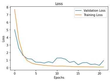
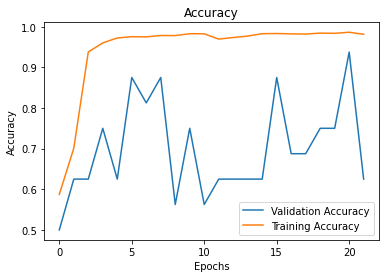
Overfitting or high variance in machine learning models occurs when the accuracy of your training dataset, the dataset used to “teach” the model, is greater than your testing accuracy. In terms of ‘loss’, overfitting reveals itself when your model has a low error in the training set and a higher error in the testing set. You can identify this visually by plotting your loss and accuracy metrics and seeing where the performance metrics converge for both datasets.
Loss vs. Epoch Plot
Accuracy vs. Epoch Plot
Overfitting indicates that your model is too complex for the problem that it is solving, i.e. your model has too many features in the case of regression models and ensemble learning, filters in the case of Convolutional Neural Networks, and layers in the case of overall Deep Learning Models. This causes your model to know the example data well, but perform poorly against any new data.
This is annoying but can be resolved through tuning your hyperparameters, but first, let’s start by making sure our data is divided into well-proportioned sets.
Splitting the Data
For a deep learning model, I recommend having 3 datasets: training, validation, and testing. The validation set should be used to fine-tune your model until you’re satisfied with its performance, then switch to the testing data to train the best version of your model. First, we’ll import the necessary library:
from sklearn.model_selection import train_test_split
Now let’s talk proportions. My ideal ratio is 70/10/20, meaning the training set should be made up of ~70% of your data, then devote 10% to the validation set, and 20% to the test set, like so,
# Create the Validation Dataset
Xtrain, Xval, ytrain, yval = train_test_split(train_images, train_labels_final, train_size=0.9, test_size=0.1, random_state=42)# Create the Test and Final Training Datasets
Xtrain, Xtest, ytrain, ytest = train_test_split(Xtrain, ytrain, train_size=0.78, random_state=42)
You will need to perform two train_test_split() function calls. The first call is done on the initial training set of images and labels to form the validation set. We’ll call the parameters random_state to keep consistency in results when running the function, and test_size to note that we want the size of our validation set to be 10% of the training data, and train_size to set it equal to the remaining percentage of data to be 90%.
This can be omitted by default as python is smart enough to do the math. The variables Xval and yval refer to our validation images and labels. On the second call, we will generate our testing dataset from our newly formed training data Xtrain and ytrain. We will repeat the above, but this time we will set the newest training set to be 78% of the previous and assign the newest dataset to the same variable as the previous for consistency. Meanwhile, we will assign the testing data to Xtest for the test images and test for the label data.
Now we’re ready to begin modeling. Refer to my previous blog to get a deep dive into the initial CNN setup. We will start on the second model assuming our first turned out like the image above. We will use the techniques below:
Regularization
Weight Initialization
Dropout Regularization
Weight Constraints
Other
Regularization
Regularization optimizes a model by penalizing complex models, therefore minimizing loss and complexity. Thus this forces our neural network to be simpler. Here we will use an L2 regularizer, as it is the most common and is more stable than an L1 regularizer. Here we’ll add a regularizer to the second and third layers of our network with a learning rate (lr) of 0.01.
Weight initialization sets up the weights vector for all neurons for the first time before the training process begins. Choosing the correct weights is crucial because we want to get as close as possible to the global minimum of our cost function in an adequate amount of time. In this iteration of our model we will use a He initialization:
# Input Layer of the 3rd Model
model3.add(layers.Conv2D(32, (3, 3), activation=’relu’, kernel_initializer=’he_normal’, input_shape=(96, 96, 3)))
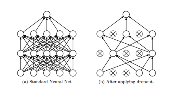
Dropout Regularization
Dropout regularization ignores a random subset of units in a layer while setting their weights to zero during that phase of training.
The ideal rate for the input and hidden layers is 0.4, and the ideal rate for the output layer is 0.2. See below:
A weight constraint checks the size of the network weights and rescales them if the size exceeds a predefined limit. The weight constraint works as required. Below we are using the constraint unit_norm, which forces the weights to have a magnitude of 1.0.
Another route is to increase the resolution of all of the photos by increasing the size. You can do this by calling new image data generators for the train, validation, and test datasets. See below how I increased the dimensions of the photos from (96 x 96) to (128 x 128):
# Import the Original Training Dataset
train_gen2 = ImageDataGenerator(rescale=1./255).flow_from_directory(train_dir, target_size=(128,128), batch_size=15200)# Import the Original Validation Dataset
val_gen2 = ImageDataGenerator(rescale=1./255).flow_from_directory(val_dir, target_size=(128,128), batch_size=16)
# Import the Original Testing Dataset
test_gen2 = ImageDataGenerator(rescale=1./255).flow_from_directory(test_dir, target_size=(128,128), batch_size=624)
About the Author
Erica Gabriel
Data Rules Everything Around Me (D.R.E.A.M). Mechanical Engineer & Project Manager turned Data Scientist, using data to build equitable and sustainable solutions to help the systemically oppressed.
A verification link has been sent to your email id
If you have not recieved the link please goto
Sign Up page again
Loading...
Please enter the OTP that is sent to your registered email id
Loading...
Please enter the OTP that is sent to your email id
Loading...
Please enter your registered email id
This email id is not registered with us. Please enter your registered email id.
Don't have an account yet?Register here
Loading...
Please enter the OTP that is sent your registered email id
Loading...
Please create the new password here
We use cookies on Analytics Vidhya websites to deliver our services, analyze web traffic, and improve your experience on the site. By using Analytics Vidhya, you agree to our Privacy Policy and Terms of Use.Accept
Privacy & Cookies Policy
Privacy Overview
This website uses cookies to improve your experience while you navigate through the website. Out of these, the cookies that are categorized as necessary are stored on your browser as they are essential for the working of basic functionalities of the website. We also use third-party cookies that help us analyze and understand how you use this website. These cookies will be stored in your browser only with your consent. You also have the option to opt-out of these cookies. But opting out of some of these cookies may affect your browsing experience.
Necessary cookies are absolutely essential for the website to function properly. This category only includes cookies that ensures basic functionalities and security features of the website. These cookies do not store any personal information.
Any cookies that may not be particularly necessary for the website to function and is used specifically to collect user personal data via analytics, ads, other embedded contents are termed as non-necessary cookies. It is mandatory to procure user consent prior to running these cookies on your website.