AdaBoost and Gradient Boost – Comparitive Study Between 2 Popular Ensemble Model Techniques
Overview
At the end of this article, you will be able to-
- Understand the working and math behind two ML techniques namely AdaBoost and Gradient Boost.
- Similarities and differences between AdaBoost and Gradient Boost algorithms.
A brief introduction on Ensemble Techniques
Combining two or more classifiers or models and making a prediction (either through voting for classification or average for numerical) to increase the performance accuracy is called Ensemble models. They are more useful and proficient when the model is unstable(flexible) resulting in high variance between different sample sets taken out of the population. The basic intuition behind this is to expose the model to maximum variance within the given dataset itself. Here for simplicity, decision tree models are used as base classifiers.
AdaBoost
This is a type of ensemble technique, where a number of weak learners are combined together to form a strong learner. Here, usually, each weak learner is developed as decision stumps (A stump is a tree with just a single split and two terminal nodes) that are used to classify the observations.
In contrary to the random forest, here each classifier has different weights assigned to it based on the classifier’s performance (more weight is assigned to the classifier when accuracy is more and vice-verse), weights are also assigned to the observations at the end of every round, in such a way that wrongly predicted observations have increased weight resulting in their probability of being picked more often in the next classifier’s sample. So, the consecutive training set depends on their previous training set, and hence correlation exists between the built trees.
Thus, Adaboost increases the predictive accuracy by assigning weights to both observations at end of every tree and weights(scores) to every classifier. Hence, in Adaboost, every classifier has a different weightage on final prediction contrary to the random forest where all trees are assigned equal weights.
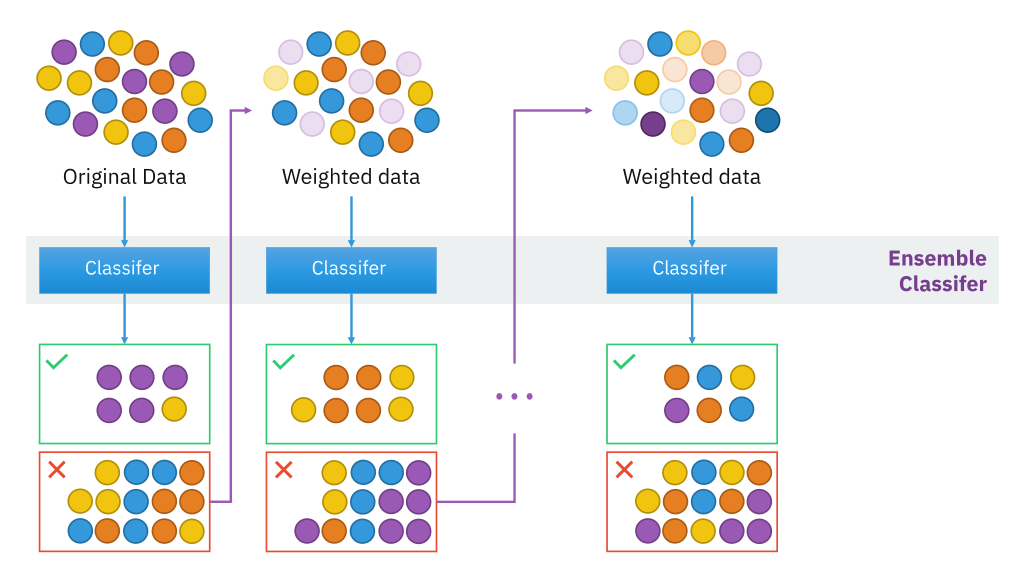
Source:https://en.wikipedia.org/wiki/Boosting_(machine_learning)#/media/File:Ensemble_Boosting.svg
Mathematically, the error rate of a classifier is given by-
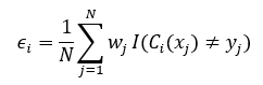
Where wj is weight
assigned to each observation of training set Di [ Initially, for the first classifier, it is equally distributed]. I am nothing but the Identity function to filter out wrong predictions made by the classifier.
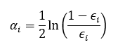
The importance of classifier is given by-

The mechanism of updating weights to observation is-
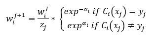
The function exp(-alpha(i)) reduces the weight of correctly classified observation and exp(alpha(i)) increases the weight of misclassified observation, thus, increasing their chance of getting picked. zj is the normalization factor that is used to reassign weights of observation such that all weights sum up to 1.
The final prediction of each observation is made by aggregating the weighted average of the prediction made by each classifier. AdaBoost might result in overfitting. Hence, no. of trees should be checked and restricted.
Gradient Boosting Machine (GBM)
Just like AdaBoost, Gradient Boost also combines a no. of weak learners to form a strong learner. Here, the residual of the current classifier becomes the input for the next consecutive classifier on which the trees are built, and hence it is an additive model. The residuals are captured in a step-by-step manner by the classifiers, in order to capture the maximum variance within the data, this is done by introducing the learning rate to the classifiers.
By this method, we are slowly inching in the right direction towards better prediction (This is done by identifying negative gradient and moving in the opposite direction to reduce the loss, hence it is called Gradient Boosting in line with Gradient Descent where similar logic is employed). Thus, by no. of classifiers, we arrive at a predictive value very close to the observed value.
Initially, a tree with a single node is built which predicts the aggregated value of Y in case of regression or log(odds) of Y for classification problems after which trees with greater depth are grown on previous classifier’s residuals. Usually, in GBM, every tree is grown with 8-32 terminal nodes, and around 100 trees are grown. Learning rates are given as constant for every tree so that the model takes small steps in the right direction to capture the variance and train the classifier on it. Unlike Adaboost, here all the trees are given equal weights.
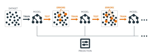
Source: Hands-on Machine Learning with R
Let us run through step by step execution of the GBM algorithm,
- Input Data (xi, yi) where i = 1(1) n where
n being total no. of observations in the sample and differentiable loss
function L(Yi , F(x)).
For a regression problem, there are different variants of loss function like Absolute Loss, Huber Loss. Generally, we use the squared residual loss for the reason of computational simplicity. For a classification problem, the loss function is estimated from negative log-likelihood which is converted to log(odds).
-
Step 1: Initialize the model with a constant value
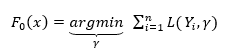
where L is the loss function and Yi is observed and gamma is the predicted value. This is the first tree that is grown with a single leaf after which trees with greater depth are built. Usually, it is the average of Yi values for regression and log(odds) value for classification.
-
Step 2: For m = 1 to M where M is the total no. of trees to be built
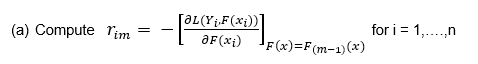
This equation gives the negative gradient of each observation for every tree which includes the previous classifier’s predicted values.
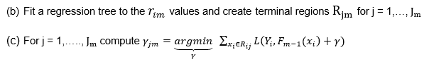
This equation finds the aggregated predicted values of each terminal nodes of every tree with minimized loss function including previous’ learners prediction
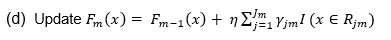
Where n is the learning rate of every tree which reduces the effect of each tree on final prediction thereby increasing the accuracy.
-
Step 3: Output FM (x)
Thus, GBM makes the final prediction by cumulating inputs from all the trees.
Comparison between AdaBoost and Gradient Boost
| S.No | Adaboost | Gradient Boost |
| 1 | An additive model where shortcomings of previous models are identified by high-weight data points. | An additive model where shortcomings of previous models are identified by the gradient. |
| 2 | The trees are usually grown as decision stumps. | The trees are grown to a greater depth usually ranging from 8 to 32 terminal nodes. |
| 3 | Each classifier has different weights assigned to the final prediction based on its performance. | All classifiers are weighed equally and their predictive capacity is restricted with learning rate to increase accuracy. |
| 4 | It gives weights to both classifiers and observations thus capturing maximum variance within data. | It builds trees on previous classifier’s residuals thus capturing variance in data. |
References
1. Hastie, Trevor, Tibshirani, Robert, Friedman, Jerome, The Elements of Statistical Learning, Data Mining, Inference, and Prediction, Second Edition.
2. Michael Steinbach, Pang-Ning Tan, and Vipin Kumar, Introduction to Data Mining.


%23/media/File:Ensemble_Boosting.svg)
"All classifiers are weighed equally and their predictive capacity is restricted with learning rate to increase accuracy" - Could you please elaborate on this point? How are classifiers weighted equally and how learning learning rate influences accuracy of each classifier? Thanks in advance!!