Bajaj Finance Stock Price Prediction in Python

Introduction

The motivation behind This article comes from the combination of passion(about stock markets) and a love for algorithms. Who doesn’t love to make money and if you know the algorithms that you have learned will or can help you make money(not always), why not explore it.

Business Usage: The particular problem pertains to forecasting, forecasting can be of sales, stocks, profits, and demand for new products. Forecasting is a technique that uses historical data as inputs to make informed estimates that are predictive in determining the direction of future trends. Businesses utilize forecasting to determine how to allocate their budgets or plan for anticipated expenses for an upcoming period of time.

Forecasting has got its own set of challenges like which variables affect a certain prediction, can there be an unforeseen circumstance(like COVID) that will render my predictions inaccurate. So forecasting is easier said than done, there is less than a % chance that the observed value will be equal to the predicted value. In that case, we try to minimize the difference between actual and predicted values.

The Data

I have downloaded the data of Bajaj Finance stock price online. I have taken the data from 1st Jan 2015 to 31st Dec 2019.1st Jan 2019 to 31st Dec 2019, these dates have been taken for prediction/forecasting. 4 years of data have been taken as training data and 1 year as test data. I have taken an open price for prediction.

EDA :

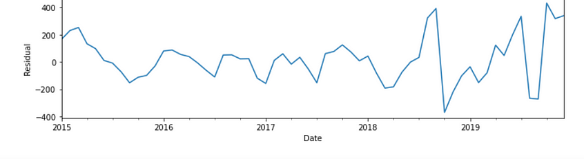
The only EDA that I have done is known as seasonal decompose, to break it up into Observed, trend, seasonality, and residual components

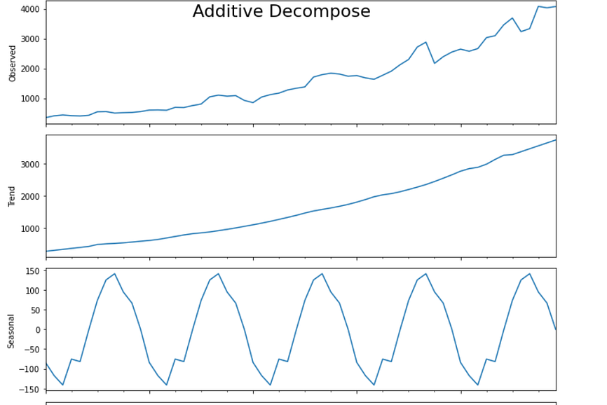
The stock price always tends to show an additive trend because seasonality does not increase with time.

Now when we decompose a time series, We get:

1. Observed: The average value in the series.
2. Trend: The increasing or decreasing value in the series, the trend is usually a long term pattern, it spans for over more than a year.
3. Seasonality: The repeating short-term cycle in the series. In time-series data, seasonality is the presence of variations that occur at specific regular intervals less than a year, such as weekly, monthly, or quarterly. …Seasonal fluctuations in a time series can be contrasted with cyclical patterns.
4. Residual: The component which is left after level, trend, and seasonality has been taken into consideration.

Model Building:

ARIMA(AutoRegressive Integrated Moving Average): This is one of the easiest and effective machine learning algorithms for performing time series forecasting. ARIMA consists of 3 parts, Auto-Regressive(p), Integrated or differencing(d), and Moving Average(q).

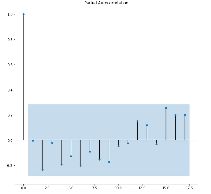
Auto-Regressive: This part deals with the fact that the current value of the time series is dependent on its previous lagged values or we can say that the current value of the time series is a weighted average of its lagged value. It is denoted by p, so if p=2, it means the current value is dependent upon the previous two of its lagged values. Order p is the lag value after which the PACF plot crosses the upper confidence interval for the first time. We use the PACF(Partial autocorrelation function)to find the p values. The reason we use the PACF plot is that it only shows residuals of components that are not explained by earlier lags. If we use ACF in place of PACF, it shows a correlation with lags that are far in fast, hence we will use the PACF plot.

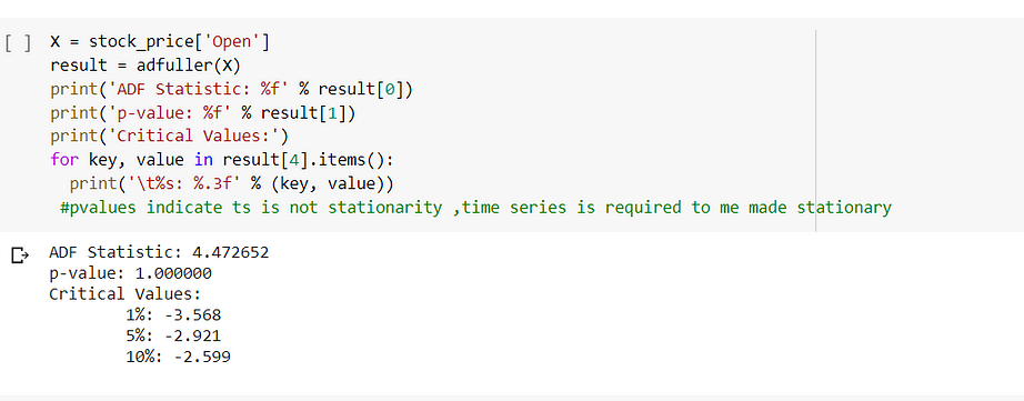
Integrated(d): One of the important features of the ARIMA model is that the time series used for modeling should be stationary. By stationarity I mean, the statistical property of time series should remain constant over time, meaning it should have a constant mean and variance. The trend and seasonality will affect the value of the time series at different times.

How to check for stationarity?

1. One simple technique is to plot and check.
2. We have statistical tests like ADF tests(Augmented Dickey-Fuller Tests).ADF tests the null hypothesis that a unit root is present in the sample. The alternative hypothesis is different depending on which version of the test is used but is usually stationarity or trend-stationarity. It is an augmented version of the Dickey-Fuller test for a larger and more complicated set of time series models. The augmented Dickey-Fuller (ADF) statistic, used in the test, is a negative number. The more negative it is, the stronger the rejection of the hypothesis that there is a unit root at some level of confidence.So if value p value<alpha(significance) ,we will reject the null hypothesis,i.e presence of unit root.

How to make time-series stationarity?

1. Differencing: The order of differencing (q) refers to the no of times you difference the time series to make it stationary. By difference, I mean you subtract the current value from the previous value. After Differencing you again perform the ADF test to check whether the time series has become stationary or you can plot and check.
2. Log Transformation: We can make the time series stationary by doing a log transformation of the variables. We can use this if the time series is diverging.

Moving Average(q)

In moving average the current value of time series is a linear combination of past errors. We assume the errors to be independently distributed with the normal distribution. Order q of the MA process is obtained from the ACF plot, this is the lag after which ACF crosses the upper confidence interval for the first time, As we know PACF captures correlations of residuals and the time series lags, we might get good correlations for nearest lags as well as for past lags. Why would that be?

Since our series is a linear combination of the residuals and none of the time series own lag can directly explain its presence (since it’s not an AR), which is the essence of the PACF plot as it subtracts variations already explained by earlier lags, its kind of PACF losing its power here! On the other hand, being a MA process, it doesn’t have the seasonal or trend components so the ACF plot will capture the correlations due to residual components only.

Model Building:

I had used auto Arima to build the model. Auto ARIMA is available in pmdarima. After fitting the test set I got an output of ARIMA(0,0,0) which is commonly known as white noise. White noise means that all variables have the same variance (sigma²) and each value has a zero correlation with all other values in the series.

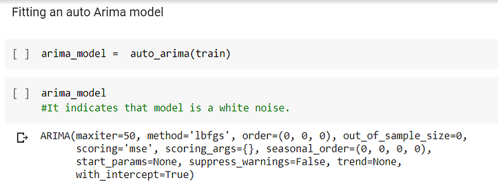
After fitting the Arima model, I printed the Summary and got the below.

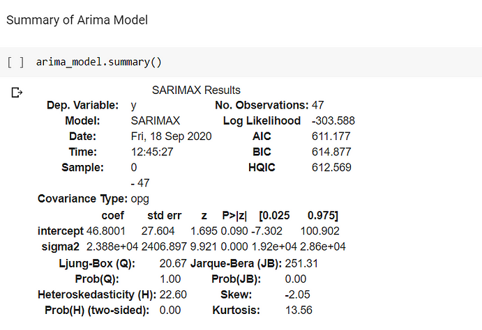
Log-Likelihood

The log-likelihood value is a simpler representation of the maximum likelihood estimation. It is created by taking logs of the previous value. This value on its own is quite meaningless, but it can be helpful if you compare multiple models to each other. Generally speaking, the higher the log-likelihood, the better. However, it should not be the only guiding metric for comparing your models!

AIC

AIC stands for Akaike’s Information Criterion. It is a metric that helps you evaluate the strength of your model. It takes in the results of your maximum likelihood as well as the total number of your parameters. Since adding more parameters to your model will always increase your value of the maximum likelihood, the AIC balances this by penalizing for the number of parameters, hence searching for models with few parameters but fitting the data well. Looking at the models with the lowest AIC is a good way to select to best one! The lower this value is, the better the model is performing.

BIC

BIC (Bayesian Information Criterion) is very similar to AIC, but also considers the number of rows in your dataset. Again, the lower your BIC, the better your model works. BIC induces a higher penalization for models with complicated parameters compared to AIC.

Both BIC and AIC are great values to use for feature selection, as they help you find the simplest version with the most reliable results at the same time.

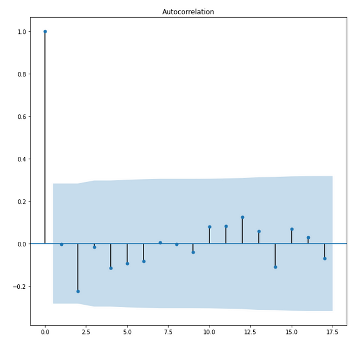
Ljung Box

The Ljung–Box test is a type of statistical test of whether any of a group of autocorrelations of a time series are different from zero. Instead of testing randomness at each distinct lag, it tests the “overall” randomness based on a number of lags and is, therefore, a portmanteau test.

Ho: The model shows the goodness of fit(The autocorrelation is zero)

Ha: The model shows a lack of fit(The autocorrelation is different from zero)

My model here satisfies the goodness of fit condition because Probability(Q)=1.

Heteroscedasticity

Heteroscedasticity means unequal scatter. In regression analysis, we talk about heteroscedasticity in the context of the residuals or error term. Specifically, heteroscedasticity is a systematic change in the spread of the residuals over the range of measured values.

My residuals are heteroscedastic in nature since Probability(Heteroskadisticy)=0.

Tests For Heteroscedasticity

Brusche Pagan test:

The Breusch-Pagan-Godfrey Test (sometimes shortened to the Breusch-Pagan test) is a test for heteroscedasticity of errors in regression. Heteroscedasticity means “differently scattered”; this is opposite to homoscedastic, which means “same scatter.” Homoscedasticity in regression is an important assumption; if the assumption is violated, you won’t be able to use regression analysis.

Ho: Residuals are homoscedastic

Ha: Residuals are heteroscedastic in nature.

Goldfeld Quandt Test:

The Goldfeld Quandt Test is a test used in regression analysis to test for homoscedasticity. It compares variances of two subgroups; one set of high values and one set of low values. If the variance differs, the test rejects the null hypothesis that the variances of the errors are not constant.

Although Goldfeld and Quandt described two types of tests in their paper (parametric and non-parametric), the term “Quandt Goldfeld test” usually means the parametric test. The assumption for the test is that the data is normally distributed.

The test statistic for this test is the ratio of mean square residual errors for the regressions on the two subsets of data. This corresponds to the F-test for equality of variances. Both the one-tailed and two-tailed tests can be used.

Forecasting Using Arima:

The metrics we use to see the accuracy of the model are RMSE.

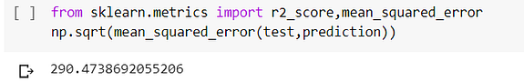
Let us see the forecasting Using ARIMA.

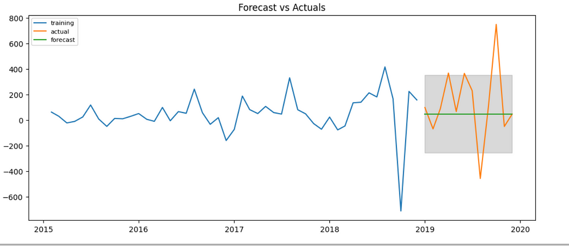
Here the forecast values are constant because it’s an ARIMA(0,0,0) model.

Prediction Using Simple Exponential Smoothing

The simplest of the exponentially smoothing methods are naturally called simple exponential smoothing. This method is suitable for forecasting data with no clear trend or seasonal pattern.

Using the naïve method, all forecasts for the future are equal to the last observed value of the series. Hence, the naïve method assumes that the most recent observation is the only important one, and all previous observations provide no information for the future. This can be thought of as a weighted average where all of the weight is given to the last observation.

Using the average method, all future forecasts are equal to a simple average of the observed data. Hence, the average method assumes that all observations are of equal importance, and gives them equal weights when generating forecasts.

We often want something between these two extremes. For example, it may be sensible to attach larger weights to more recent observations than to observations from the distant past. This is exactly the concept behind simple exponential smoothing. Forecasts are calculated using weighted averages, where the weights decrease exponentially as observations come from further in the past — the smallest weights are associated with the oldest observations.

So large value of alpha(alpha denotes smoothing parameter)denotes that recent observations are given higher weight and a lower value of alpha denoted that more weightage is given to distant past values.

Modelling Using Simple Exponential Smoothing:

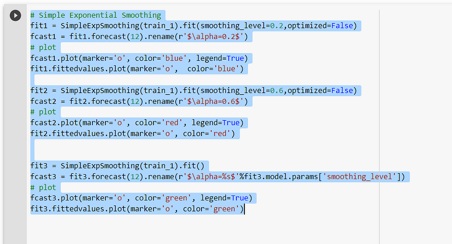
By modeling Using Simple Exponential Smoothing, we have taken 3 cases.

In fit1, we explicitly provide the model with the smoothing parameter α=0.2

In fit2, we choose an α=0.6

In fit3, we use the auto-optimization that allows statsmodels to automatically find an optimized value for us. This is the recommended approach.

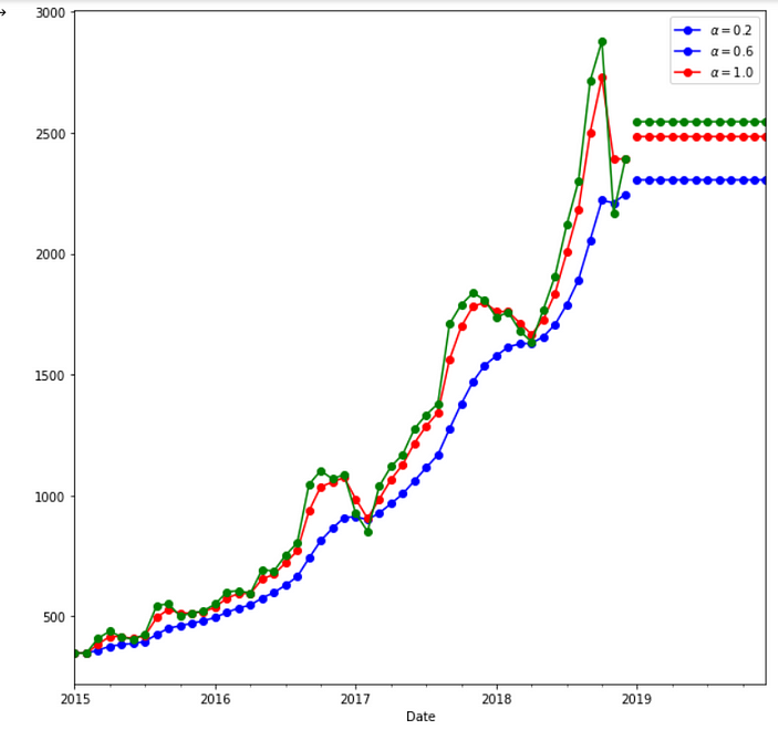
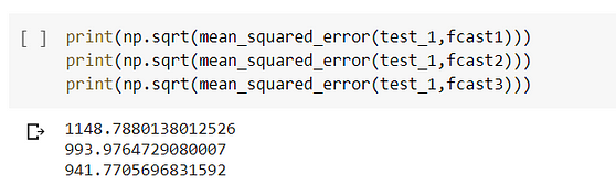
The best output is given when alpha=1, indicating recent observations are given the highest weight.

Holt’s Model

Holt extended simple exponential smoothing to allow the forecasting of data with a trend. (alpha for level and beta * for trend). The forecasts generated by Holt’s linear method display a constant trend(either upward or downward). Due to this, we tend to over forecast-hence we use a concept of damped trend. It dampens the trend to a flat line in the near future.

Modeling Using Holt’s Model:

Under this, we took three cases

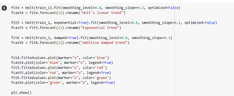
1.In fit1, we explicitly provide the model with the smoothing parameter α=0.8, β*=0.2.

2.In fit2, we use an exponential model rather than Holt’s additive model(which is the default).

3.In fit3, we use a damped version of the Holt’s additive model but allow the dampening parameter ϕ to be optimized while fixing the values for α=0.8, β*=0.2.

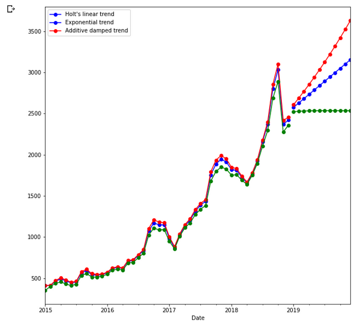
Prediction Using Holt’s model

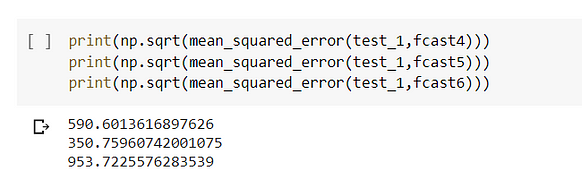
The lowest value of RMSE is when alpha=0.8 and smoothing-slope=0.2 when the model is the exponential model in nature.

Holt’s Winter Model

Holt and Winters extended Holt’s method to capture seasonality. The Holt-Winters seasonal method comprises the forecast equation and three smoothing equations. It has three parameters alpha which is the level, Beta* which is the trend, and gamma which is the seasonality. The additive method is preferred when the seasonal variations are roughly constant through the series, while the multiplicative method is preferred when the seasonal variations are changing proportionally to the level of the series.

Modeling Using Holt’s Winter Model

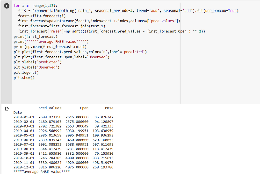
1.In fit1, we use additive trend, additive seasonal of period season_length=4, and a Box-Cox transformation.

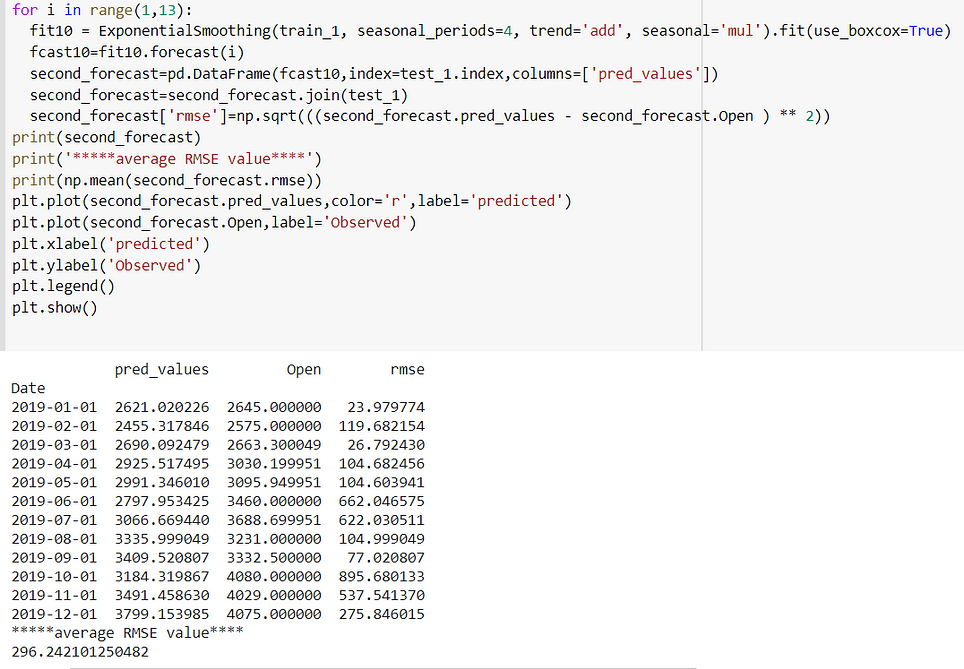
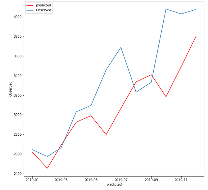
2.In fit2, we use additive trend, multiplicative seasonal of period season_length=4, and a Box-Cox transformation.

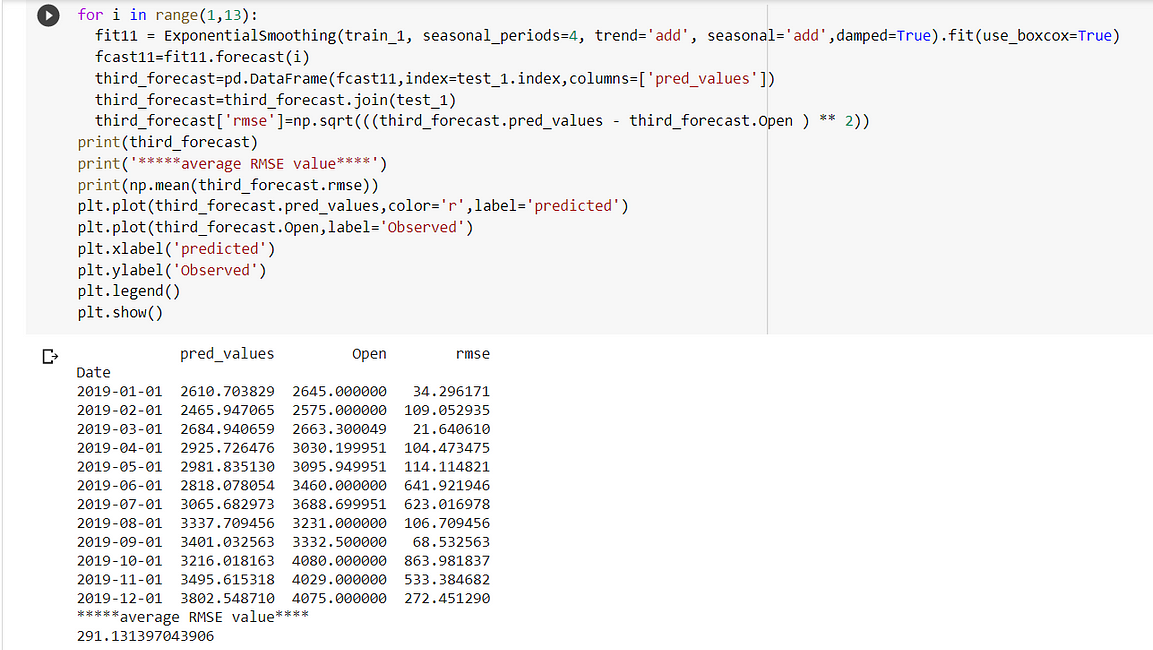
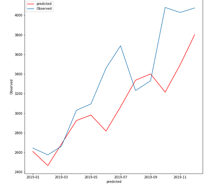
3.In fit3, we use additive damped trend, additive seasonal of period season_length=4, and a Box-Cox transformation.

4.In fit4, we use multiplicative damped trend, multiplicative seasonal of period season_length=4, and a Box-Cox transformation.

Box-Cox Transformation: A Box-Cox transformation is a transformation of a non-normal dependent variable into a normal shape. Normality is an important assumption for many statistical techniques; if your data isn’t normal, applying a Box-Cox means that you are able to run a broader number of tests.

Case1:

In fit1, we use additive trend, additive seasonal of period season_length=4, and a Box-Cox transformation.

Case 2:

In fit2, we use additive trend, multiplicative seasonal of period season_length=4, and a Box-Cox transformation.

Case 3:

In fit3, we use additive damped trend, additive seasonal of period season_length=4, and a Box-Cox transformation.

Case 4:

In fit4, we use multiplicative damped trend, multiplicative seasonal of period season_length=4, and a Box-Cox transformation.

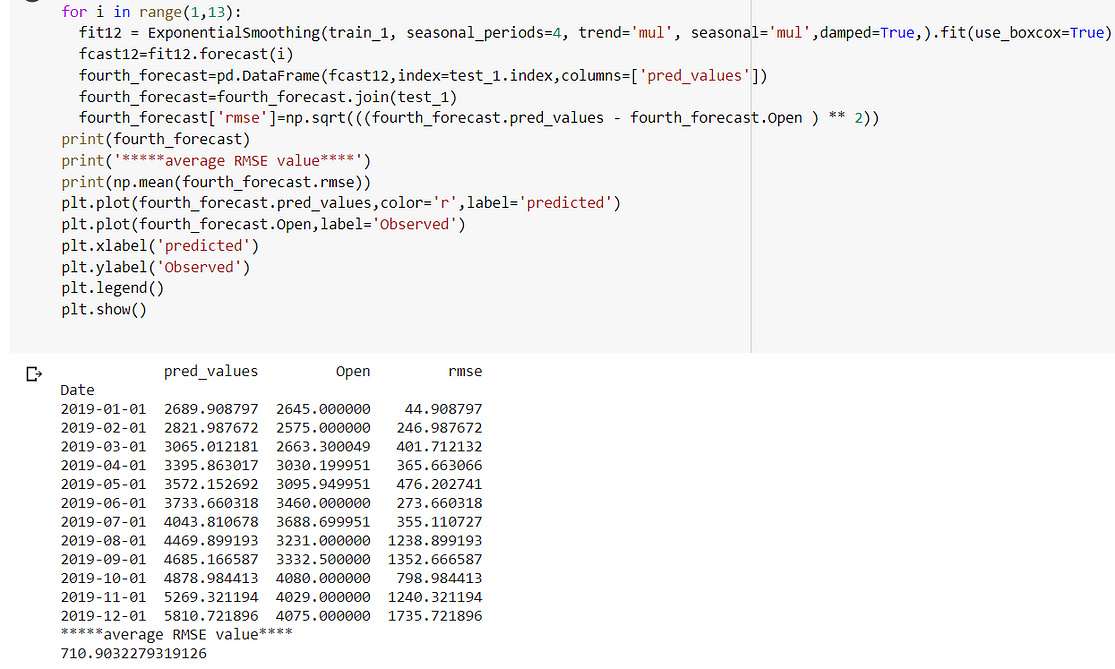
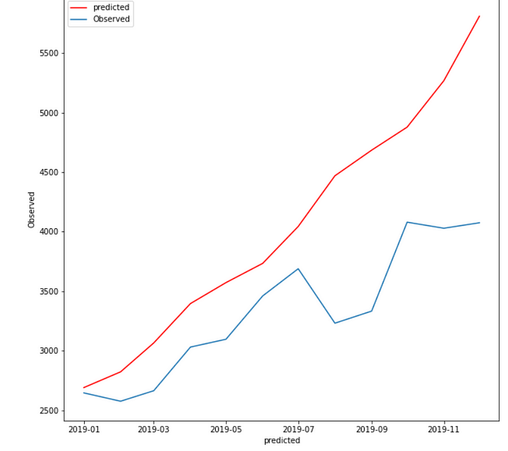
Best Model:

The holt winter is giving me the lowest RMSE(281.91) when trend and seasonality are additive.

Linear Regression

Up Next I applied the Linear Regression Model with Open Price as my dependent variable.Steps involved in Linear Regression

1. Check for missing Values.
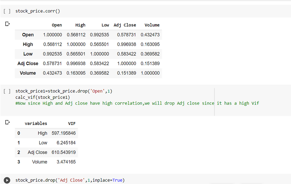
2. Check for multicollinearity, if there is high multicollinearity -calculate VIF, the variable with the highest VIF, drop that variable. Repeat the process until all the variables are not affected by multicollinearity.

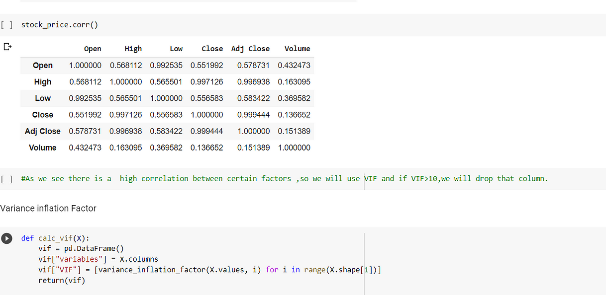
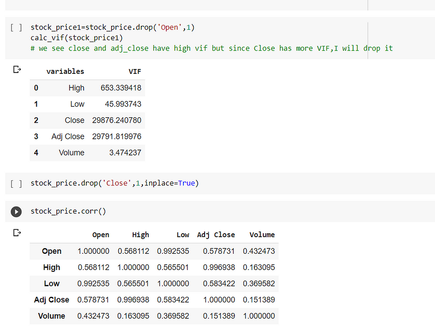
In the above (fig 1) we see that adj_close and close both have very high VIF then we saw that Close has more VIF then we will drop it. Post that we will again check the correlation and we see that Adj Close and High have a high correlation.

In the above fig(fig 2) we see that Adj close has a higher vif value than High, So we will drop that variable.

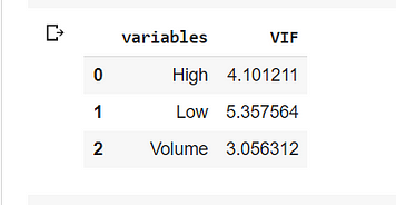
Now we can perform the modeling part. Let us look at the OLS regression.

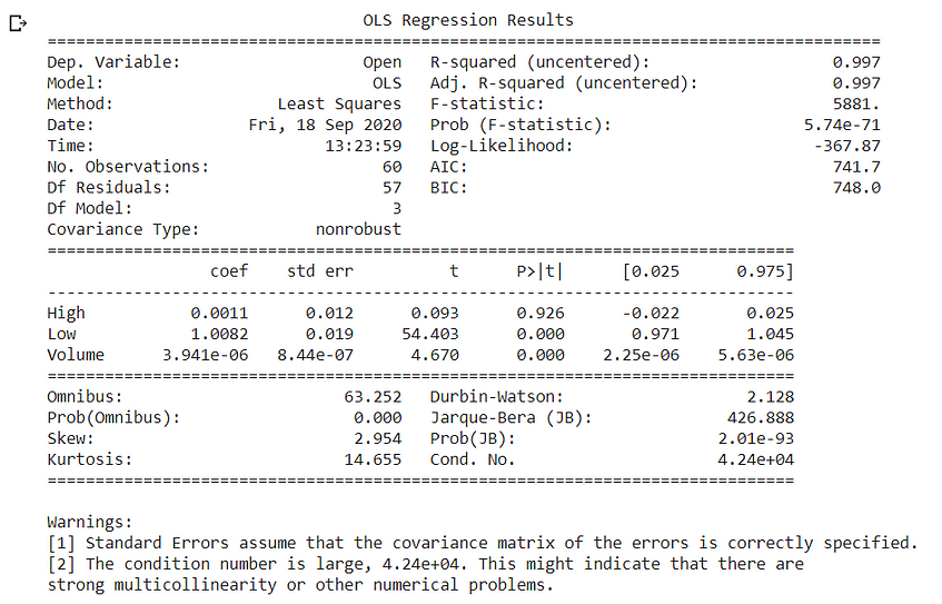
OLS Analysis:

1. Significant Variables: As per the p values, significant variables are Low, Volume.
2. Omnibus: Omnibus is a test for skewness and kurtosis. In this case, the omnibus is high and the probability of omnibus is zero, indicating residuals are not normally distributed.
3. Durbin Watson: It is a test for autocorrelation at AR(1) lag.

The Hypotheses for the Durbin Watson test are:
H0 = no first order autocorrelation.
H1 = first order correlation exists.
(For a first-order correlation, the lag is a one-time unit).

In this case, autocorrelation is 2.1 indicating negative autocorrelation.

Heteroskadistic Tests:

Brusche Pagan Test.

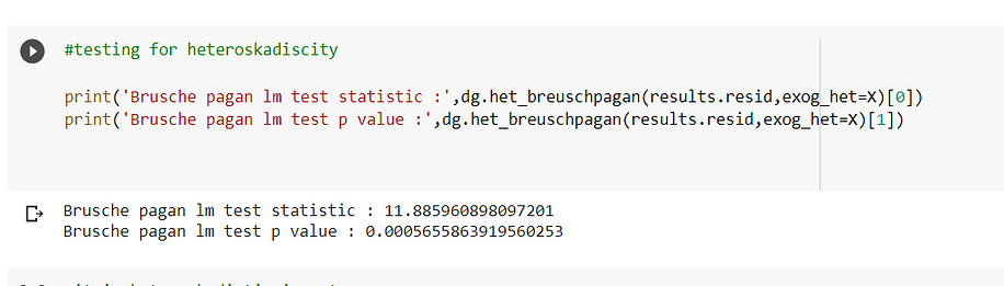
As per the above test, our residuals or errors are heteroskedastic in nature. Heteroskedasticity is a problem because it makes our model less inefficient because there will be some unexplained variance that cannot be explained by any other model.

RMSE:

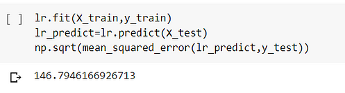
Error: 4.4%, which is quite acceptable.

Random Forest:

Next, I build a model using Random Forest Regressor. Firstly I built a model with the given hyperparameters.

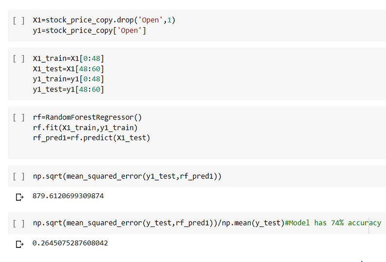
Error rate:26% which is quite high and RMSE is 879.612

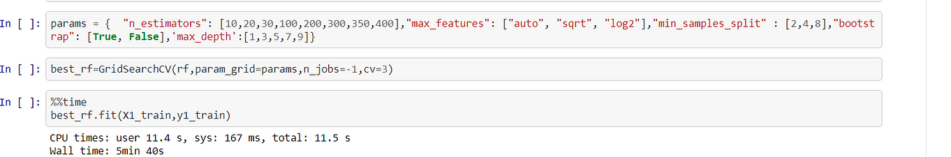
Next, we tuned our hyperparameters using Grid search.

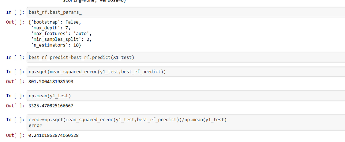
So After tuning the hyperparameters, I saw that RMSE scored had decreased and error has become 24% (which is still very high ) as compared to linear regression.

Support Vector Regressor

Linear Kernel:

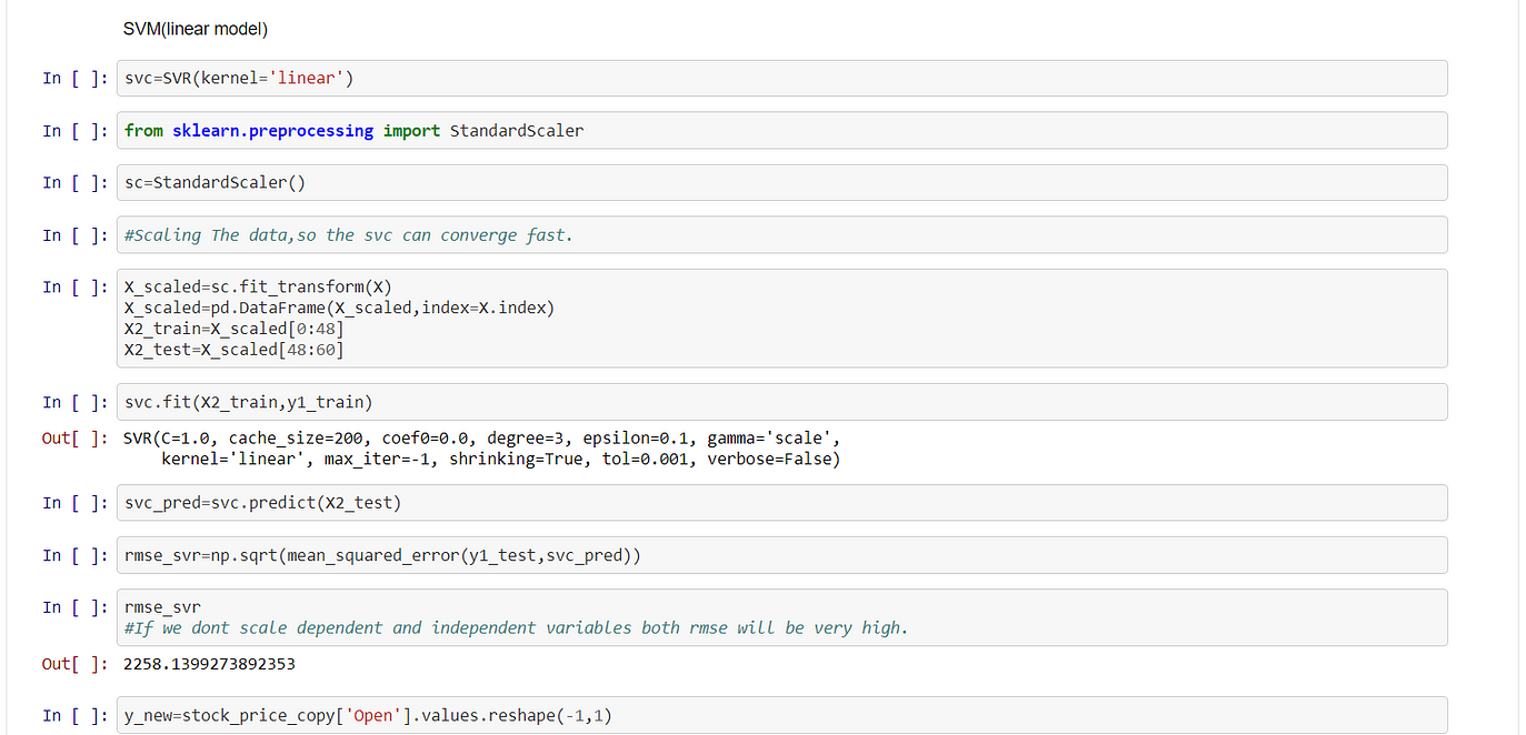
In Svm Scaling is a necessary condition otherwise it takes a lot of time to converge. It is necessary to scale both the independent and dependent variables. Post prediction we need to do reverse scaling, otherwise, the scale of predicted variables and the test set will be different.

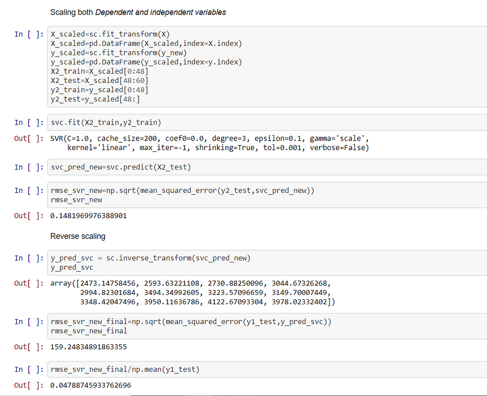
After building the model we see that RMSE score is 159.24 and the error is 4.7% which is quite close to Linear Regression.

Support Vector Regression(RBF KERNEL)

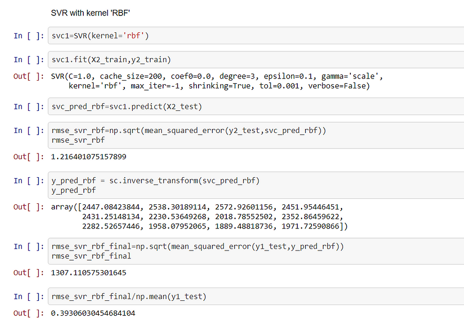
In the above snippet, we actually see that when we use RBF kernel our RMSE score increased drastically to 1307, and error increased to 39.3%. So RBF kernel is not suitable for this model.

Support Vector Regression(Polynomial KERNEL)

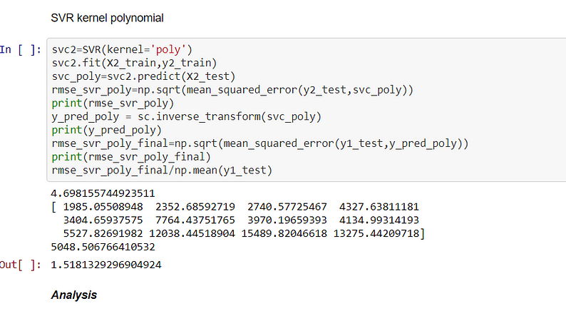
From the above output, it is clear polynomial kernel is not suitable for this dataset because RMSE(5048.50) is very high and the error is 151.8%. So this gives us a clear picture that data is linear in nature.

Analysis

Out of all the models, we have applied, the best model is Linear Regression(lowest RMSE score of 146.79) and the error is 4.45%

You can find out my code here(Github Link:https://github.com/neelcoder/Time-Series)

You can reach me at LinkedIn(https://www.linkedin.com/in/neel-roy-55743a12a/)

About the Author

Neel Roy

As an executive with over 4 years of experience in the BFSI Industry, I offer a record of success as a key contributor in the process & sales operations management that solved business problems in consumer targeting, market prioritization, and business analytics. My background as a marketer, export & import/ LC process expert, combined with my technical acumen has positioned me as a valuable resource in delivering and enhancing solutions.

I have successfully completed Data Science Certification from Jigsaw Academy, 1st level of Certification from IIBA (International Institute of Business Analysis), and currently pursuing PGP Data Science from Praxis Business School, seeking an assignment to utilize my skills and abilities in the field of Data Science. I have good knowledge of Python, SQL, R & Tableau, and Data Processing.

I am equally comfortable in the business and technical realms, communicating effortlessly with clients and key stakeholders, I leverage skills in today’s technologies spanning data analytics & data mining, primary research, consumer segmentation, and market analysis. I engage my passion, creativity, and analytical skills to play a vital role in facilitating the company’s success and helping to shape the organization’s future.