Overview
- Understand the limitations of linear regression for a classification problem, the dynamics, and mathematics behind logistic regression.
- Understand how GLM is used for classification problems, the use, and derivation of link function, and the relationship between the dependent and independent variables to obtain the best solution.
- Learn how a classification problem converts to optimization and how the probabilities are estimated using maximum likelihood.
- Understand the importance of optimal cut-off and how to predict the classes as the final solution.
Introduction
In machine learning, a classification problem is grouping the data into predefined classes. An event is predicted where the response is categorical in nature or in other words, predicts the class for a given set of data. This can be performed on both structured or unstructured data. Structured data simply means where the target is already defined and unstructured or unlabeled data means where the target is unknown. The focus of this article is on structured data.
Some of the instances of classes are: for an insurance company to categorize an insurance claim as fraud or genuine; a product manufactured is defective or not defective; for a telecom provider whether the customer will churn (i.e. leave the company) or not churn; whether a patient is diagnosed with cancer or not and alike. This is a binary classification where there are two classes.
When there are more than two classes such as having high, medium, or low risk is a form of multi-class classification. The iris dataset having classes of flowers as Setosa, Versicolor, Virginica is an example of multi-class classification. In this article, will be working through a problem to predict whether the person is likely to have heart disease or not.

Table of Contents
- Challenges with Linear Regression for classification problems and the need for Logistic Regression
- The general form of Sigmoid Curve and GLM
- Concept and Derivation of Link Function
- Estimation of the coefficients and probabilities
- Conversion of Classification Problem into Optimization
- The output of the model and Goodness of Fit
- Defining the optimal threshold
Challenges with Linear Regression for classification problems and the need for Logistic Regression
In a classification problem, the target variable(Y) is categorical and the predictors (X) can be numerical or categorical. For understanding purposes, will take one independent variable (Age) to classify Y into a person likely to have heart disease or not, where having the disease is 1 and not having the disease is 0.
| Age (X) | Target (Y) |
| 76 | 1 |
| 63 | 0 |
| 41 | 1 |
| 48 | 0 |
| 37 | 1 |
| 56 | 1 |
| 62 | 1 |
| 39 | 0 |
| 70 | 0 |
| 65 | 0 |
The goal is to achieve this for which would need an equation of Y = F(X1, X2, X3… Xn) that will establish a mathematical relationship between the Y and Xs. Now, the question arises can linear regression be used to find the best-fit line and classify Y?
To perform Linear Regression following assumptions must be followed:
- Y should follow a normal distribution
- Y and X must have a linear relationship
The reasons Linear Regression cannot be used in a classification problem is because of the challenges that have with our present data:
- What relationship does the data hold?
From the table above, can say if a person’s age is more then the person will have the disease, or if the person is younger the person does not have the disease. Is it possible to have a linear relationship in this scenario? The output may be a linear line however, that wouldn’t be the best fit line using linear regression. Hence, how to get the best possible solution?
- Is Y (the target variable) following Normal distribution?
In the problem, Y is a categorical variable that has two categories and is following binomial distribution, hence violates the assumption that Y must follow normal distribution for Linear Regression.
- In addition to this, there would be some relationship between X and Y in classification problems, however, that wouldn’t be linear according to the Linear Regression assumption.
- Moreover, the output from Linear Regression can have negative values and values greater than one as well. This will exceed the range of predicted values for Y from 0 and 1.
On the left side of the graph below, can see that the classes (disease or not disease) lie on X and Y axis and by fitting a Linear Regression, the best-fit line y = mx + c wouldn’t give the best solution as the straight line will misclassify between diseases and non-diseases. So now, how to achieve the best solution? There are many possibilities for achieving the best solution. The one that will use and talk about is the Sigmoid curve (S-curve).
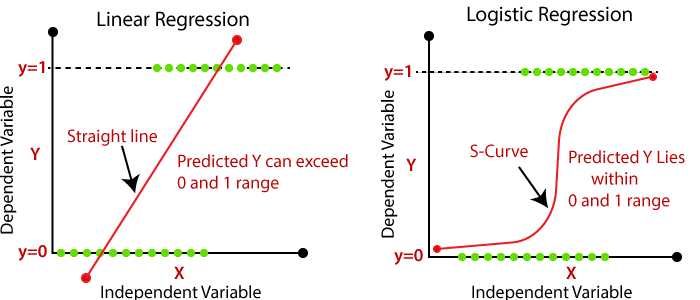
source: https://static.javatpoint.com/tutorial/machine-learning/images/linear-regression-vs-logistic-regression.png
With the help of the Sigmoid curve, can classify between the disease and non-disease classes as illustrated in the right side of the graph below. Intuitively, can understand that the best fit line is S-curve as compared to the linear line in such cases. This leads us to ask how to come up with the S-curve?
There are two ways to achieve the S-curve (Sigmoid Curve):
- One way is through Logistic Regression:
P = e(b0 + b1*x)/ (1 + e(b0 + b1*x)) - The second way is through Probit Regression:
P = e(-1/F(X))
The focus of this article is on Logistic Regression and will explore the above-mentioned expression in detail below.
The objective of Logistics Regression is to achieve a solution between X and Y in such a way to get the S-curve that is the best fit line in a classification model.
The general form of the Sigmoid Curve and GLM
Every curve has a mathematical equation. In Logistic Regression, the general form of the S-curve is:
P = e(b0 + b1*x)/ (1 + e(b0 + b1*x))
or
P = 1/(1 + e-(b0 + b1*x))
Using this general form equation will be achieving our objective of finding a classifier to distinguish between a person likely to have heart disease or not. After applying some mathematical operations on this, get the following:
P/(1-P) = e(b0 + b1*x)
Taking log on both sides, the equation becomes:
Log(P/(1-P)) = b0 + b1*x
Now, p/1-p is nothing but the odds ratio. The odds ratio is the ratio of the probability of success to the probability of failure.
Odds = P(Y=1)/P(Y=0)
P(Y=1) or p is the probability of success of an event.
P(Y=0) or (1-p) is the probability of failure of an event.
Event: Person has heart disease
The reason the gears are switched towards probability is that the output of Logistic Regression is always a probability or in other words it predicts likelihood. As probabilities are always between 0 and 1, henceforth this also solves one of the limitations of predicted values for Y exceeding from the range of 0 and 1 that had occurred on applying Linear Regression for classification problems.
The equation becomes:
Log(odds) = b0 + b1*x
Concept and Derivation of Link Function
Every distribution can be converted into normal distribution by applying the transformation. Here, assigning log(odds) as Z:
Z = Logit(Y) = log(odds) = Log (p/1-p) = b0 + b1*x
What does it mean to apply a transformation on the target variable Y in Logistic regression?
It means to come up with Logit(Y) = Log(p/1-p) = Log(odds) that follows Normal distribution and find p and (1-p) by applying log transformation on the odds ratio.
How is the transformation applied?
By applying the Link function of Logit. What is Logit? It is Log(p/1-p) which is the link function. The link function is nothing but the transformation that applies and by doing so has now generalized to the linear model concept. Hence, instead of using the Y variable, used Log of odds and this helped to achieve the relationship between X and Link (Y) that is Log(p/1-p).
The purpose of the generalized linear model was:
- To find the link function that converts Y into normally distributed data, and
- The relationship between Y & X must be of S-curve (Sigmoid curve).
Applying transformation on the target variable Y that makes Z = Logit(Y) = Log(p/1-p) = Log(odds) follows Normal distribution, henceforth can apply Linear Regression to compute the betas.
Estimation of the coefficients and probabilities
As was in Linear Regression, for various values of b0 and b1 could have a linear equation but for those specific values of b0 and b1 which would give minimum the sum of squared errors will be the best fit line.
Similarly, in Logistic Regression, can have various S-curves for different values of b0 , b1 hence infinite S-curves are possible. So, this leads to a very important question that is how to estimate the coefficients or the betas which provide the best-fit curve for logistic regression? To find the values of betas b0 , b1, b2….. bn would need some algorithm i.e. some mathematical equation, correct?
The mathematical equation that has is:
Log(odds) = b0 + b1*x
With the help of Linear Regression and using the relationship that got above from the S-curve, will compute the values of the coefficients. The Sigmoid -curve is dependent on the betas cause the equation of S-curve is P = 1/ (1 + e-(b0 + b1*x )) and with the help of betas would compute the probability of P(Y=1) that will help to separate the 0s and 1s i.e. the people having heart disease and not having heart disease.
The reason can use Linear Regression is because the right-hand side of the equation is b0 + b1*x and have transformed the left-hand side of the equation so that Z follows Normal distribution and henceforth satisfies the assumptions to apply Linear Regression which is 1) Y must follow Normal distribution and 2) X and Y should have a linear relationship.
So, have used the general form of S-curve and the Generalized Linear Model (GLM) concept to derive the Logit function and use which can apply Linear Regression to estimate the betas in Z = Log(p/1-p) = b0 + b1*x. This is appropriate when there is only one independent variable. But, in reality, the data will n.
ever have only one independent variable. It will certainly have a lot of predictors and also a mix of both categorical and numerical independent (x) variables. In that case, how to compute the betas?
First, let’s address how to estimate betas and probabilities for different types of features:
- Categorical variables: In the dataset, have a variable called ca: number of major vessels colored by flourosopy (0-4) which can be bucketed based on the count of vessels that have been colored by fluorosopy. Thereby, get the frequencies for people having zero, one, two, three or four vessels colored; for each of these separate into 1s and 0s and find the probability of 1s and probability of 0s then apply the log transformation on p/1-p i.e. log of odds that gives the transformed Logit(Y) and apply Linear Regression on this to find the betas. This is illustrated below:
ca N #1’s #0’s P(Y=1) P(Y=0) Odds Log(odds) 0 175 134 41 0.7657 0.2343 3.2683 0.5143 1 65 21 44 0.3231 0.6769 0.4773 -0.3212 2 38 7 31 0.1842 0.8158 0.2258 -0.6463 3 20 3 17 0.1500 0.8500 0.1765 -0.7533 4 5 4 1 0.8000 0.2000 4.0000 0.6021 Total 303 210 93 - Numerical variables: For one of the numerical variables: age, shown below the first step is to convert the numerical X into bins and find the frequencies for each of the bins, then for each of the bins find the 1s and 0s and the odds ratio. Henceforth, the process is the same to apply the log transformation to get the Logit(Y) which would follow a normal distribution and apply Linear Regression to find the betas.
Age N #1’s #0’s P(Y=1) P(Y=0) Odds Log(odds) 30-40 16 11 5 0.6875 0.3125 2.2000 0.3424 40-50 72 50 22 0.6944 0.3056 2.2727 0.3565 50-60 125 65 60 0.5200 0.4800 1.0833 0.0348 60-70 80 32 48 0.4000 0.6000 0.6667 -0.1761 70+ 10 6 4 0.6000 0.4000 1.5000 0.1761 Total 303 164 139
Conversion of classification problem into Optimization
Now, let’s dive into how to compute betas for many independent variables. The steps that have followed until now to calculate the probabilities for one single predictor would need to be repeated and hence the manual estimation for each and every variable surely is a tedious task. Therefore, will be using Optimization for the computation of betas
Some of you may be wondering that the goal was to find a classifier, decision boundary for the data, and then how and why have landed to Optimization?
In the data, the known variables are the independent X values and the unknown values are the betas. Optimization will help us to find the values of the unknowns (which are the coefficients or the betas of the independent variables) and will return those values that minimize the objective function. But, what is the objective function in the classification technique, Logistic Regression?
Here’s a question for you all, when can you say that the model is good? or, in other words, can conclude what values of the betas or the coefficient values are the best solution?
The model is said to be good when P(Y=1) is high meaning that there are higher chances of the person having heart disease and P(Y=0) is low indicating that there are fewer chances for the person to have heart disease. This is more of intuitive understanding.
To mathematically formulate this, the probabilities of P(Y=1) and P(Y=0) are computed. Now, estimate what will be the value of a person has a disease as 1 and a person not having the disease as 0. In other words,find this value [Y*P(Y=1) + (1-Y)*P(Y=0)]. The coefficients that give the maximum value of [Y*P(Y=1) + (1-Y)*P(Y=0)] are the best betas and hence will provide the best solution. This concept is known as the Maximum Likelihood.
| Age | Target | P(Y=1) | P(Y=0) | Y*P(Y=1)+(1-Y)*P(Y=0) | -(Y*P(Y=1)+(1-Y)*P(Y=0)) | -(Y*log(P(Y=1))+(1-Y)*log(P(Y=0))) |
| 76 | 1 | 0.6 | 0.4 | 0.6 | -0.6 | 0.2218 |
| 63 | 0 | 0.3 | 0.7 | 0.7 | -0.7 | 0.1549 |
| 41 | 1 | 0.4 | 0.6 | 0.4 | -0.4 | 0.3979 |
| 48 | 0 | 0.2 | 0.8 | 0.8 | -0.8 | 0.0969 |
| 37 | 1 | 0.6 | 0.4 | 0.6 | -0.6 | 0.2218 |
| 56 | 1 | 0.3 | 0.7 | 0.3 | -0.3 | 0.5229 |
| 62 | 1 | 0.2 | 0.8 | 0.2 | -0.2 | 0.6990 |
| 39 | 0 | 0.7 | 0.3 | 0.3 | -0.3 | 0.5229 |
| 70 | 0 | 0.1 | 0.9 | 0.9 | -0.9 | 0.0458 |
| 65 | 1 | 0.7 | 0.3 | 0.7 | -0.7 | 0.1549 |
| 5.1 | -5.1 | 3.4068 |
Maximum likelihood: It is calculating the likelihood of the event happening and this likelihood of the event of a person having heart disease must be maximum. That is, have to maximise the sum of [Y*P(Y=1) + (1-Y)*P(Y=0)].
P(Y=1) = e(b0 + b1*x1 + b2*x2 + ….+ bn*xn)/ (1 + e(b0 + b1*x1 + b2*x2 + ….+ bn*xn))
The objective function in Logistic Regression is to convert the maximization problem F(x) to the Minimization problem of -F(x). So, the concept is to find the values of x that come with the next iteration of x for which the F(x) must decrease. This comes from the concept of Gradient Descent. To get the values of x, would need to use partial derivatives. The derivatives of exponential value results in exponential which is time-consuming hence to avoid that would take log values henceforth would convert the Minimise likelihood to Minimise Negative Log Likelihood. The reason for doing this is to minimize the convergence time using the negative log likelihood estimation.
The objective function now becomes: – { [Y*log P(Y=1)] + [(1-Y)*log P(Y=0)]} which converts this to an optimization problem.
Maximise : F(x) = sum [Y*P(Y=1) + (1-Y)*P(Y=0)] —- > Maximise likelihood
Minimise : – F(x) = – {sum [Y*P(Y=1) + (1-Y)*P(Y=0)]} —- > Minimise likelihood
Why compute this? This is the process of estimation of betas in Logistic Regression. Using this method to come up with the maximum values corresponding to the event of a person having heart disease and this eventually helps to differentiate between 0s and 1s that is the classifier or the decision boundary and lead to the final solution that is the best fit curve which is Sigmoid (S-curve).
When building any model, there are two imperative things:
- What is the accuracy of the model?
- How quickly does the model converge?
We’ll look into the accuracy of the model in some time. To converge the model quickly had converted the objective function of maximizing likelihood to minimize negative log likelihood.
Output of the Model and Goodness of Fit
The resultant of Logistic Regression is:
- the Sigmoid Curve , and
- Probability ofP = P(Y=1) = e(b0 + b1*x)/ (1 + e(b0 + b1*x))
or
P = P(Y=1) = 1/ (1 +e(b0 + b1*x))meaning the solution achieved is the probability p i.e P(Y=1) which is the probability i.e. likelihood of an event happening.
Taking the story forward, have computed the betas that help us in estimating the probabilities of an event happening and not happening and this will separate the ones from the zeros and define the classifier. However, that’s not the ultimate goal.
The end goal is to predict whether the next (or new) person will have heart disease or not. In other words, is this new person one or zero? This brings to the question, how to use these probabilities to predict if the person is one or zero?? All the exercises up until this point have been on the training dataset. Now, shall move towards the testing (or unseen) data.
Goodness of fit:
these metrics indicate how good the model is. The metrics are divided as follows:
- Based on the probability as an output
- Concordance, Discordance, SomerceD, Gamma
- Area Under the curve
- Based on the predicted categories
- Confusion Matrix
- Classification report (Accuracy, Sensitivity, Specificity, precision, recall, f1 score)
Metrics based on probability as an output:
We get the following predicted values:
| Actual | Predicted | cut-off=50% | |
| Id | Target | P(Y=1) | Pred |
| 1 | 1 | 0.6 | 1 |
| 2 | 0 | 0.3 | 0 |
| 3 | 0 | 0.4 | 0 |
| 4 | 0 | 0.2 | 0 |
| 5 | 1 | 0.6 | 1 |
| 6 | 1 | 0.3 | 0 |
| 7 | 1 | 0.2 | 0 |
| 8 | 0 | 0.7 | 1 |
| 9 | 0 | 0.1 | 0 |
| 10 | 1 | 0.3 | 0 |
| 0.5 |
As discussed above, the model is good for those values where the probability is high that it’s more likely for the person to have the disease and less likely for the person to not have heart disease. Therefore, this indicates that the likelihood of a non-disease person P(Y=0) must always be less than the likelihood of a person having heart disease P(Y=1). Based on this have separated the 1s and 0s and created the following table that segregates the people having a disease or not based on a 50% cut-off (is also the default threshold in sklearn).
In this, comparing every non-disease person with every diseased person i.e. comparing 25 pairs and bucketing these pairs based on P(Y=1) greater than, less than or equal to P(Y=0).
| Disease | ||||||
| P(Y=1) | 0.6 | 0.6 | 0.3 | 0.2 | 0.3 | |
| P(Y=0) | No Disease | 1 | 5 | 6 | 7 | 10 |
| 0.3 | 2 | |||||
| 0.4 | 3 | |||||
| 0.2 | 4 | |||||
| 0.7 | 8 | |||||
| 0.1 | 9 |
The pairs having P(Y=1)greater than P(Y=0) are colored in green and are called concordant pairs; the pairs where P(Y=1) is less than P(Y=0) are colored in orange and are called dis-concordant pairs and the pairs that have same probability for success and failure of the event are tied pairs and are yellow in color. Taking the proportion of each set of pairs out of the total 25 pairs, get the following results:
| % | ||
| Concordant pairs | 13 | 0.52 |
| Discordant pairs | 9 | 0.36 |
| Tied pairs | 3 | 0.12 |
| Gini/Somerce D | C-D | 0.16 |
| Gamma | (C-D)/(C+D) | 0.1818181818 |
- C: Concordance
- D: Discordance
- T: Ties
Estimating the concordance, discordance leads to computation of Sommerce D/Gini and Gamma, which are metrics of the goodness of fit.
Gini or Sommerce D is calculated as the difference between concordance and discordance divided by the total of concordance, discordance and ties.
Gamma is computed as the difference between concordance and discordance divided by the total of concordance and discordance, or in other words, Gamma is the change in concordance and discordance.
When concordance is high then the discordance and ties are less. High concordance, high Sommere D, or high Gamma, all indicate the model is good suggesting how much the model is differentiating between 1s and 0s.
Metrics based on the predicted categories:
In this, compute how many values are classified as 1s and how many are classified as 0s. This leads to the confusion matrix.
Confusion Matrix:
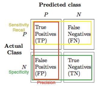
source: https://newbiettn.github.io/images/confusion-matrix-noted.jpg
- True Positive (TP) refers to the number of predictions where the classifier correctly predicts the positive class as positive.
- False Positive (FP) is the number of predictions where the classifier incorrectly predicts the negative class as positive. It is also known as the Type I Error.
- True Negative (TN) refers to the number of predictions where the classifier correctly predicts the negative class as negative.
- False Negative (FN) is the number of predictions where the classifier incorrectly predicts the positive class as negative. It is also known as Type II Error.
In the dataset, the model is predicting a person likely to have heart disease, here too many type II errors is not advisable. The false-negative (ignoring the probability of disease when there actually is one) is more dangerous than a False Positive in this case. Hence, in order to increase sensitivity, the threshold can be lowered.
Classification report
Recall/Sensitivity:
Recall is the ability to correctly detect. It tells us how many of the actual positive cases were the model able to predict correctly. Recall is a useful metric in cases where false Negative is of higher concern.
Precision/Specificity:
Precision is the ability to correctly predict. It tells us how many of the correctly predicted cases actually turned out to be positive. Precision is a useful metric in cases where false positive is a higher concern than false negatives.
F1 score:
F1-score is a harmonic mean of precision and recall, and it gives a combined idea about these two metrics. It is maximum when precision is equal to recall.
How to define optimal cut-off?
Now, have said that want to distinguish between 1s and 0s which is done based on the probabilities but what if define a threshold say the cutoff for P(Y=1) is defined as 0.45 that any new person having P(Y=1) equal or more than 0.45 in 1 and less than 0.45 is defined as 0. However, what if the threshold changes? This will not only change the cut-off value but also change the prediction for whether the new person is having a disease or not having the disease. Hence, would need to come up with an optimal cutoff which will help to predict the new person and also to calculate the scoring.
There are different approaches to get the optimal cutoffs:
- Percentage of ones in the Y variable (not
- Confusion Matrix (which has been discussed above)
- AUC Curve
- Decile Analysis
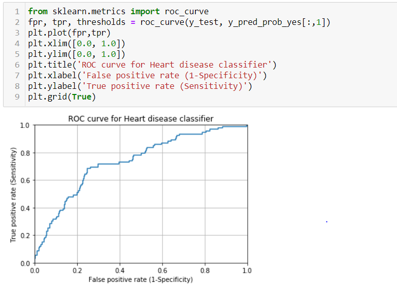
Receiver Operating Characteristic curve (ROC curve) :
A common way to visualize the trade-offs of different thresholds is by using a ROC curve, a plot of the true positive rate (true positives/ total positives) or in other words Sensitivity against the false positive rate (false positives/total negatives) or (1-Specificity) for all the possible choices of thresholds. In a nutshell, a ROC curve is a graph that shows the performance of a classification model at all the possible thresholds.
A model with good classification accuracy must significantly have more true positives than false positives at all thresholds. The optimum position for the roc curve is towards the top left corner where the specificity and sensitivity are at optimum levels. The following graph depicts this:
Area Under The Curve (AUC)
The area under the ROC curve quantifies model classification accuracy; the higher the area, the greater the disparity between true and false positives, and the stronger the model in classifying members of the training dataset.
An area of 0.5 corresponds to a model that performs no better than random classification and a good classifier stays as far away from that as possible. An area of one is ideal. The closer the AUC to one the better.
This leads to the concluding question: how to identify the optimal cut-off?
- Based on the confusion matrix: the threshold that gives the highest sensitivity or accuracy or f1-score is the best cut-off.
- According to the ROC curve: the cut-off that gives high sensitivity and low (1-specificity) is the best model. In case, there is a tie between two such models then AUC works as the tie-breaker and the model with high AUC is the better model.
Endnotes/Summary
The goal of any classification problem is to find a decision boundary or classifier that separates 1s and 0s. We saw in depth the limitations of Linear Regression in light of the classification problem and why Logistic regression fits the bill. We have also explored the concept of generalized linear models that can be used in this kind of problem.
Using the general form of Sigmoid curve, which gives the best fit line, had derived the link function i.e. the Logit of the odds ratio. That is in order to get the link function, discuss the relationship between the target variable and the predictors. Going forward, we saw how to convert the classification problem into an optimization problem and solve it. It is also imperative to understand the following:
- The probabilities were computed to estimate the betas, and
- These probabilities were calculated with the help of Linear Regression.
Post building the model, what is the output of the model? Once the probabilities are achieved how will obtain the optimal cut-off and also discussed how to identify and predict the classes post obtaining the optimal cut-off. As discussed, once we know the mathematical equation and the thresholds, we can apply new data and predict for new people.
Hi there! I am Neha Seth. I work as a Data Scientist in Larsen & Toubro Infotech (LTI). I hold a Postgraduate Program in Data Science & Engineering from the Great Lakes Institute of Management and a Bachelors in Statistics. I have been featured as Top 10 Most Popular Guest Authors in 2020 on Analytics Vidhya (AV).
My area of interest lies in NLP and Deep Learning. I have also passed the CFA Program. You can reach out to me on LinkedIn and can read my other blogs for AV.


Hello, can you give the code in R as well? Thank you
Hi, Apologies I wouldn't be able to provide the codes in R as I am yet to learn R language. I have worked only on Python as of now. Thank you for the interest :) Best Regards, Neha
Nicely explained..Kudos to you
Thank you Rishabh :)
Though I am not from a conventional economic background, nevertheless, being my education linkages to IT domain & public administration , this article make me understand the regression & data analytics concepts in a thoroughly manner. Thanks to the content creater !