Dimensionality Reduction using Factor Analysis in Python!
“Beauty gets the attention but personality gets the heart”. These lines portray the importance of things which lies beyond our vision. What about a Machine Learning algorithm that finds information about the inner beauty like my heart which finds the creamy layer of the Oreo despite the unappetizing outer crunchy biscuits.
INTRODUCTION
Factor analysis is one of the unsupervised machine learning algorithms which is used for dimensionality reduction. This algorithm creates factors from the observed variables to represent the common variance i.e. variance due to correlation among the observed variables. Yes, it sounds a bit technical so let’s break it down into pizza and slices.
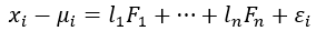
Representing features in terms of factors (Image by Author)
x is the variable and F is the factor and l is the factor loading which can also be considered as the weight of the factor for the corresponding variable. The number of factors is equal to the number of variables.
STORY-TIME
Let’s get everything more clear with an example. Let’s imagine that every one of us is now a recruiter and we want to hire employees for our business firm. The interview process has been over and for each personality of the interviewee, we have rated them out of 10. The various personalities of the interviewee are distant, relaxed, careless, talkative, lazy, etc.
There are about 32 variables. We can see that relaxed, careless, and lazy features are correlated because these persons won’t be successful. Since these variables are correlated we can try to form a factor called ‘unsuccessful behaviors’ which will explain the common variance i.e. variance due to correlation among these features.
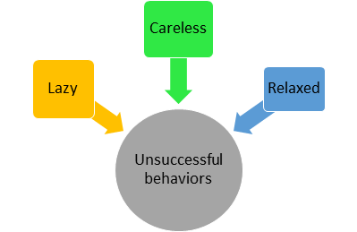
Similar or correlated features can be grouped and represented as factors (Image by Author)
The dataset and code can be downloaded from my GithubRepo
STEPS INVOLVED IN FACTOR ANALYSIS
The various steps involved in factor analysis are
- Bartlett’s Test of Sphericity and KMO Test
- Determining the number of factors
- Interpreting the factors
Make sure that you have removed the outliers, standard scaled the data and also the features have to be numeric.
I am going to implement this in python with the help of the following packages
- factor_analyzer
- numpy
- pandas
- matplotlib
BARTLETT’S TEST OF SPHERICITY
Bartlett’s test checks whether the correlation is present in the given data. It tests the null hypothesis (H0) that the correlation matrix is an Identical matrix. The identical matrix consists of all the diagonal elements as 1. So, the null hypothesis assumes that no correlation is present among the variables.
We want to reject this null hypothesis because factor analysis aims at explaining the common variance i.e. the variation due to correlation among the variables. If the p test statistic value is less than 0.05, we can decide that the correlation is not an Identical matrix i.e. correlation is present among the variables with a 95% confidence level.
from factor_analyzer.factor_analyzer import calculate_bartlett_sphericitychi2,p = calculate_bartlett_sphericity(dataframe)
print("Chi squared value : ",chi2)
print("p value : ",p)#OUTPUT:Bartlett Sphericity TestChi squared value : 4054.19037041082
p value : 0.0
Read the dataset using pandas and store the dataset in a dataframe. We have stored the dataset in a dataframe named ‘dataset’. Just simply pass the ‘dataset’ through the calculate_bartltett_sphericty function, it will test the null hypothesis and will return the chi-squared value and the p test statistic. Since the p test statistic is less than 0.05, we can conclude that correlation is present among the variables which is a green signal to apply factor analysis.
KAISER-MEYER-OLKIN (KMO) TEST
KMO Test measures the proportion of variance that might be a common variance among the variables. Larger proportions are expected as it represents more correlation is present among the variables thereby giving way for the application of dimensionality reduction techniques such as Factor Analysis. KMO score is always between 0 to 1 and values more than 0.6 are much appreciated. We can also say it as a measure of how suited our data is for factor analysis.
from factor_analyzer.factor_analyzer import calculate_kmokmo_vars,kmo_model = calculate_kmo(dataset)
print(kmo_model)#OUTPUT:
KMO Test Statistic 0.8412492848324344
Just pass the dataframe which contains information about the dataset to the calculate_kmo function. The function will return the proportion of variance for each variable which is stored in the variable ‘kmo_vars’ and the proportion of variance for the whole of our data is stored in ‘kmo_model’. we can see that our data has an overall proportion of variance of 0.84. It shows that our data has more correlation and dimensionality reduction techniques such as the factor analysis can be applied.
DETERMINING THE NUMBER OF FACTORS
The number of factors in our dataset is equal to the number of variables in our dataset. All the factors are not gonna provide a significant amount of useful information about the common variance among the variables. So we have to decide the number of factors. The number of factors can be decided on the basis of the amount of common variance the factors explain. In general, we will plot the factors and their eigenvalues.
Eigenvalues are nothing but the amount of variance the factor explains. We will select the number of factors whose eigenvalues are greater than 1.
But why should we choose the factors whose eigenvalues are greater than 1? The answer is very simple. In a standard normal distribution with mean 0 and Standard deviation 1, the variance will be 1. Since we have standard scaled the data the variance of a feature is 1. This is the reason for selecting factors whose eigenvalues(variance) are greater than 1 i.e. the factors which explain more variance than a single observed variable.
from factor_analyzer import FactorAnalyzerfa = FactorAnalyzer(rotation = None,impute = "drop",n_factors=dataframe.shape[1])fa.fit(dataframe)
ev,_ = fa.get_eigenvalues()plt.scatter(range(1,dataframe.shape[1]+1),ev)
plt.plot(range(1,dataframe.shape[1]+1),ev)
plt.title('Scree Plot')
plt.xlabel('Factors')
plt.ylabel('Eigen Value')
plt.grid()
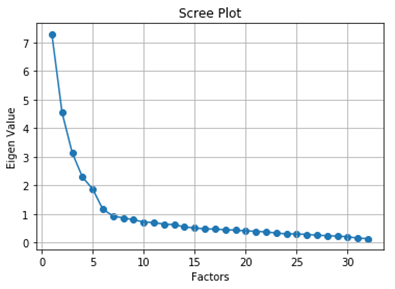
Determining Number of Factors (Image by Author)
The eigenvalues function will return the original eigenvalues and the common factor eigenvalues. Now, we are going to consider only the original eigenvalues. From the graph, we can see that the eigenvalues drop below 1 from the 7th factor. So, the optimal number of factors is 6.
INTERPRETING THE FACTORS
Create an optimal number of factors i.e. 6 in our case. Then, we have to interpret the factors by making use of loadings, variance, and commonalities.
LOADINGS
fa = FactorAnalyzer(n_factors=6,rotation='varimax')
fa.fit(dataset)
print(pd.DataFrame(fa.loadings_,index=dataframe.columns))
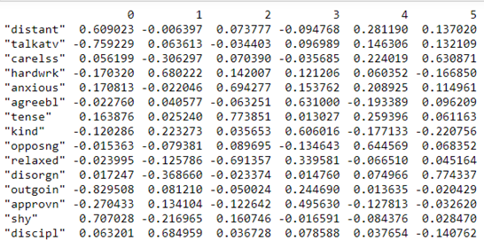
Factor Loadings (Image by Author)
Loadings indicate how much a factor explains a variable. The loading score will range from -1 to 1.Values close to -1 or 1 indicate that the factor has an influence on these variables. Values close to 0 indicates that the factor has a lower influencer on the variable.
For example, in Factor 0, we can see that the features ‘distant’ and ‘shy’ talkative have high loadings than other variables. From this, we can see that Factor 0, explains the common variance in people who are reserved i.e. the variance among the people who are distant and shy.
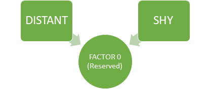
Factor 0 (RESERVED) (Image By Author)
VARIANCE
The amount of variance explained by each factor can be found out using the ‘get_factor_variance’ function.
print(pd.DataFrame(fa.get_factor_variance(),index=['Variance','Proportional Var','Cumulative Var']))
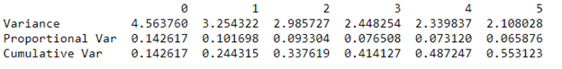
Variance Explained by Factors (Image by Author)
The first row represents the variance explained by each factor. Proportional variance is the variance explained by a factor out of the total variance. Cumulative variance is nothing but the cumulative sum of proportional variances of each factor. In our case, the 6 factors together are able to explain 55.3% of the total variance.
In unrotated cases, the variances would be equal to the eigenvalues. Rotation changes the distribution of proportional variance but the cumulative variance will remain the same. Oblique rotations allow correlation between the factors while the orthogonal rotations keep the factors uncorrelated.
COMMUNALITIES
Communality is the proportion of each variable’s variance that can be explained by the factors. Rotations don’t have any influence over the communality of the variables.
print(pd.DataFrame(fa.get_communalities(),index=dataframe.columns,columns=['Communalities']))
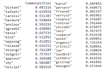
Communalities (Image by Author)
The proportion of each variable’s variance that is explained by the factors can be inferred from the above. For example, we could consider the variable ‘talkatv’ about 62.9% of its variance is explained by all the factors together.
That’s all about the factor analysis which can be used to find the underlying variance due to correlation among the observed variables like my heart which finds the creamy layer of the Oreo despite the unappetizing outer crunchy biscuits.


Hello there, Firstly, I am very grateful for your help, it's been very helpful to me. Thank you. My question is, in your "LOADINGS" section, you write "For example, in Factor 0, we can see that the features ‘distant’ and ‘shy’ talkative have high loadings than other variables. From this, we can see that Factor 0, explains the common variance in people who are reserved i.e. the variance among the people who are distant and shy." How do we know the name of the factors? You have mentioned Factor 0, but refer to this as (reserved). How did you find out that Factor 0 means reserved? Thank you, ~R