Building an ARIMA Model for Time Series Forecasting in Python
Introduction
A popular and widely used statistical method for time series forecasting is the ARIMA model. Exponential smoothing and ARIMA models are the two most widely used approaches to time series forecasting and provide complementary approaches to the problem. While exponential smoothing models are based on a description of the trend and seasonality in the data, ARIMA aim to describe the autocorrelations in the data. Before we talk about the ARIMA model Python, let’s talk about the concept of stationarity and the technique of differencing time series.

Table of contents
What is Autoregressive Integrated Moving Average (ARIMA)?
An autoregressive integrated moving average (ARIMA) model is a statistical tool utilized for analyzing time series data, aimed at gaining deeper insights into the dataset or forecasting forthcoming trends.
In this tutorial, We will talk about how to develop an ARIMA model for time series forecasting in Python.
An ARIMA model is a class of statistical models for analyzing and forecasting time series data. It is really simplified in terms of using it, Yet this model is really powerful.
ARIMA stands for Auto-Regressive Integrated Moving Average.
The parameters of the ARIMA model are defined as follows:
- p: The number of lag observations included in the model, also called the lag order.
- d: The number of times that the raw observations are differenced, also called the degree of difference.
- q: The size of the moving average window, also called the order of moving average.
Steps to Use ARIMA Model
We construct a linear regression model by incorporating the specified number and type of terms. Additionally, we prepare the data through differencing to achieve stationarity, effectively eliminating trend and seasonal structures that can adversely impact the regression model.
- Visualize the Time Series Data
Visualize the Time Series Data involves plotting the historical data points over time to observe patterns, trends, and seasonality.
- Identify if the date is stationary
Identify if the data is stationary involves checking whether the time series data exhibits a stable pattern over time or if it has any trends or irregularities. Stationary data is necessary for accurate predictions using ARIMA, and various statistical tests can be employed to determine stationarity.
- Plot the Correlation and Auto Correlation Charts
To plot the correlation and auto-correlation charts in the steps of using the ARIMA model online, you analyze the time series data. The correlation chart displays the relationship between the current observation and lagged observations, while the auto-correlation chart shows the correlation of the time series with its own lagged values. These charts provide insights into potential patterns and dependencies within the data.
- Construct the ARIMA Model or Seasonal ARIMA based on the data
To construct an ARIMA (Autoregressive Integrated Moving Average) model or a Seasonal ARIMA model, one analyzes the data to determine the appropriate model parameters, such as the order of autoregressive (AR) and moving average (MA) components. This step involves selecting the optimal values for the model based on the characteristics and patterns observed in the data.
How to Build an ARIMA Model?
Here’s how you can make an ARIMA model in simple terms using Python:
- Get Data Ready: Collect the data you want to study or predict trends in.
- Check if Data is Steady: Make sure the data doesn’t change too much over time. If it does, you might need to adjust it.
- Find Model Details: Look at the data to figure out how much you need to adjust it (if at all) and how past data affects future data. You can do this using Python libraries for time series analysis, like pandas and statsmodels.
- Fit the Model: Use the details you found to set up your ARIMA model in Python, utilizing libraries such as statsmodels.
- See How Well it Works: Check if the model matches the data well by comparing actual data with predictions made by your ARIMA model in Python.
- Predict the Future: Once the model is good, use it to guess what might happen next based on your Python ARIMA model’s predictions.
- Make it Better: If your predictions aren’t great, tweak the model in Python to improve it, perhaps by adjusting parameters or trying different algorithms.
- Check if it’s Reliable: Test your Python ARIMA model to make sure it gives accurate predictions, comparing its forecasts with actual data.
Stationarity
A stationary time series data is one whose properties do not depend on the time, That is why time series with trends, or with seasonality, are not stationary. the trend and seasonality will affect the value of the time series at different times, On the other hand for stationarity it does not matter when you observe it, it should look much the same at any point in time. In general, a stationary time series will have no predictable patterns in the long-term.
Arima Model Python
Let’s Start
import numpy as np
import pandas as pd
import matplotlib.pyplot as plt
%matplotlib inline
Defining the Dataset
In this tutorial, I am using the below dataset.
df=pd.read_csv('time_series_data.csv')
df.head()

# Updating the header
df.columns=["Month","Sales"]
df.head()
df.describe()
df.set_index('Month',inplace=True)

from pylab import rcParams
rcParams['figure.figsize'] = 15, 7
df.plot()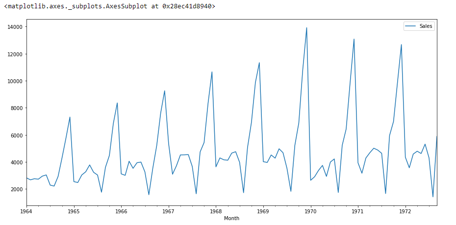
If we see the above graph then we will able to find a trend that there is a time when sales are high and vice versa. That means we can see data is following seasonality. For ARIMA first thing we do is identify if the data is stationary or non – stationary. if data is non-stationary we will try to make them stationary then we will process further.
Using Adfuller
Let’s check that if the given dataset is stationary or not, For that we use adfuller.
from statsmodels.tsa.stattools import adfullerI have imported the adfuller by running the above code.
test_result=adfuller(df['Sales'])To identify the nature of data, we will be using the null hypothesis.
- H0: The null hypothesis: It is a statement about the population that either is believed to be true or is used to put forth an argument unless it can be shown to be incorrect beyond a reasonable doubt.
- H1: The alternative hypothesis: It is a claim about the population that is contradictory to H0 and what we conclude when we reject H0.
#Ho: It is non-stationary
#H1: It is stationary
We will be considering the null hypothesis that data is not stationary and the alternate hypothesis that data is stationary.
def adfuller_test(sales):
    result=adfuller(sales)
    labels = ['ADF Test Statistic','p-value','#Lags Used','Number of Observations']
    for value,label in zip(result,labels):
        print(label+' : '+str(value) )

if result[1] <= 0.05:
    print("strong evidence against the null hypothesis(Ho), reject the null hypothesis. Data is stationary")
else:
    print("weak evidence against null hypothesis,indicating it is non-stationary ")

adfuller_test(df['Sales'])
Finding the P-value
After running the above code we will get P-value,
ADF Test Statistic : -1.8335930563276237
p-value : 0.3639157716602447
#Lags Used : 11
Number of Observations : 93
Here P-value is 0.36 which is greater than 0.05, which means data is accepting the null hypothesis, which means data is non-stationary.
Let’s try to see the first difference and seasonal difference:
df['Sales First Difference'] = df['Sales'] - df['Sales'].shift(1)
df['Seasonal First Difference']=df['Sales']-df['Sales'].shift(12)
df.head()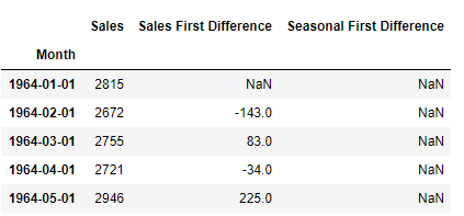
# Again testing if data is stationary
adfuller_test(df['Seasonal First Difference'].dropna())
ADF Test Statistic : -7.626619157213163
p-value : 2.060579696813685e-11
#Lags Used : 0
Number of Observations : 92Here P-value is 2.06, which means we will be rejecting the null hypothesis. So data is stationary.
df['Seasonal First Difference'].plot()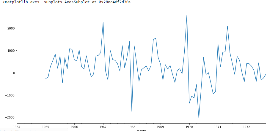
Create Auto-correlation
I am going to create auto-correlation :
from pandas.plotting import autocorrelation_plot
autocorrelation_plot(df['Sales'])
plt.show()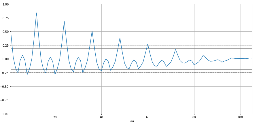
from statsmodels.graphics.tsaplots import plot_acf,plot_pacf
import statsmodels.api as sm
fig = plt.figure(figsize=(12,8))
ax1 = fig.add_subplot(211)
fig = sm.graphics.tsa.plot_acf(df['Seasonal First Difference'].dropna(),lags=40,ax=ax1)
ax2 = fig.add_subplot(212)
fig = sm.graphics.tsa.plot_pacf(df['Seasonal First Difference'].dropna(),lags=40,ax=ax2)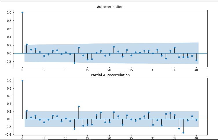
# For non-seasonal data
#p=1, d=1, q=0 or 1

from statsmodels.tsa.arima_model import ARIMA
model=ARIMA(df['Sales'],order=(1,1,1))
model_fit=model.fit()
model_fit.summary()| Dep. Variable: | D.Sales | No. Observations: | 104 |
|---|---|---|---|
| Model: | ARIMA(1, 1, 1) | Log-Likelihood | -951.126 |
| Method: | css-mle | S.D. of innovations | 2227.262 |
| Date: | Wed, 28 Oct 2020 | AIC | 1910.251 |
| Time: | 11:49:08 | BIC | 1920.829 |
| Sample: | 02-01-1964 to 09-01-1972 | HQIC | 1914.536 |
| coef | std err | z | P>|z| | [0.025 | 0.975] | |
|---|---|---|---|---|---|---|
| const | 22.7845 | 12.405 | 1.837 | 0.066 | -1.529 | 47.098 |
| ar.L1.D.Sales | 0.4343 | 0.089 | 4.866 | 0.000 | 0.259 | 0.609 |
| ma.L1.D.Sales | -1.0000 | 0.026 | -38.503 | 0.000 | -1.051 | -0.949 |
| Real | Imaginary | Modulus | Frequency | |
|---|---|---|---|---|
| AR.1 | 2.3023 | +0.0000j | 2.3023 | 0.0000 |
| MA.1 | 1.0000 | +0.0000j | 1.0000 | 0.0000 |
df['forecast']=model_fit.predict(start=90,end=103,dynamic=True)
df[['Sales','forecast']].plot(figsize=(12,8))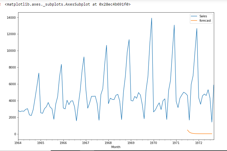
import statsmodels.api as sm
model=sm.tsa.statespace.SARIMAX(df['Sales'],order=(1, 1, 1),seasonal_order=(1,1,1,12))
results=model.fit()
df['forecast']=results.predict(start=90,end=103,dynamic=True)
df[['Sales','forecast']].plot(figsize=(12,8))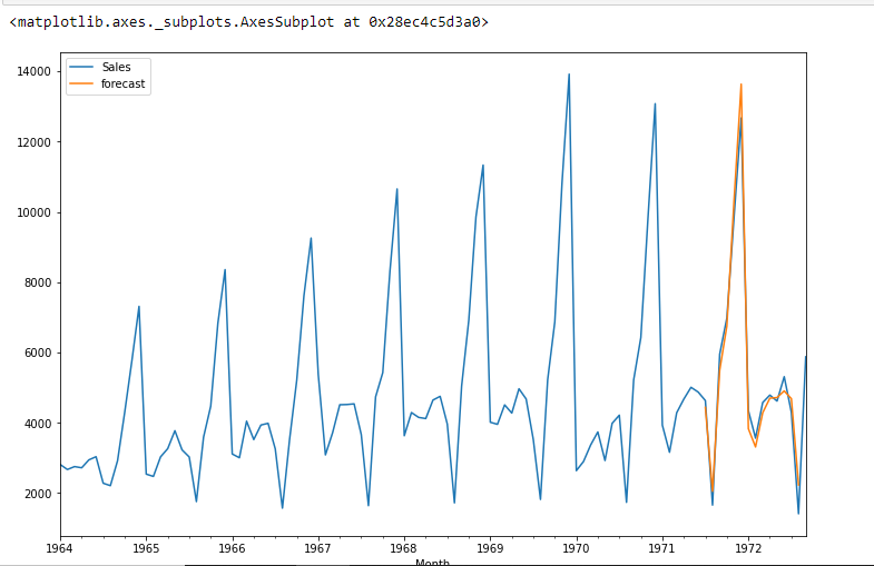
from pandas.tseries.offsets import DateOffset
future_dates=[df.index[-1]+ DateOffset(months=x)for x in range(0,24)]
future_datest_df=pd.DataFrame(index=future_dates[1:],columns=df.columns)

future_datest_df.tail()

future_df=pd.concat([df,future_datest_df])

future_df['forecast'] = results.predict(start = 104, end = 120, dynamic= True)
future_df[['Sales', 'forecast']].plot(figsize=(12, 8))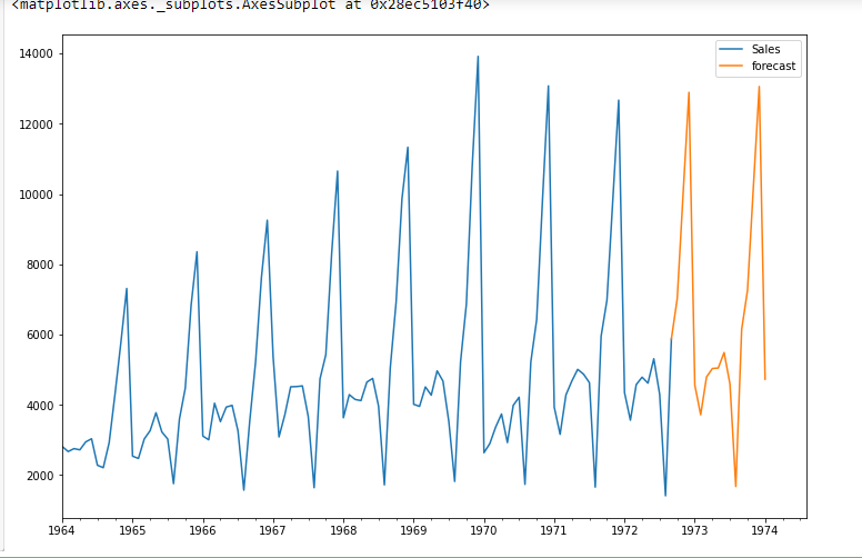
Pros and Cons of ARIMA
Here are the good and not-so-good things about using ARIMA models in Python:
Pros:
- Easy to Understand: ARIMA models in Python are pretty straightforward to grasp and use, especially if you’re familiar with time series stuff.
- Great for Stable Data: They work well when your data doesn’t change much over time, like when the average and other stats stay the same.
- Good at Predicting: ARIMA models in Python are quite reliable for telling you what might happen next based on what’s happened before, which can be super useful in business and other areas.
- Flexible: They can handle different types of data without needing to know exactly what kind of distribution it follows.
- Captures Time Patterns: ARIMA models in Python are good at picking up on how things in the past affect what happens next, which is handy for spotting trends.
Cons:
- Not Great with Changing Data: They don’t work as well if your data is all over the place or has clear patterns changing over time. You might need to do extra steps to get them to work right in Python.
- Tricky to Set Up: Figuring out the right settings for your ARIMA model in Python can be tough and might need a bit of trial and error.
- Assumes Things are Linear: ARIMA models in Python think the relationship between stuff in your data is straight and simple, which isn’t always true in real life.
- Short-Term Focus: They’re not the best at predicting stuff way far into the future. They’re more suited for short to medium-term predictions.
- Sensitive to Weird Data: ARIMA models in Python can get thrown off if there are weird outliers or unusual bits in your data, which could mess up your predictions.
Conclusion
Time Series forecasting is really useful when we have to take future decisions or we have to do analysis, we can quickly do that using ARIMA, there are lots of other Models from we can do the time series forecasting but ARIMA model is really easy to understand. If you’re interested in mastering data science techniques like ARIMA, explore enrolling in the renowned Blackbelt Plus Program. This step will enhance your skills and broaden your horizons in this dynamic field, marking the beginning of your data science journey today!
Frequently Asked Questions
A. ARIMA, or AutoRegressive Integrated Moving Average, is a time series forecasting method implemented in Python for predicting future data points based on historical time series data.
A. ARIMA and regression serve different purposes. ARIMA is suitable for time series data, while regression is used for modeling relationships between variables. The choice depends on the data and the problem.
A. No, ARIMA and regression are different. ARIMA is designed for time series forecasting, focusing on temporal patterns, while regression models the relationship between variables, irrespective of time.
A. ARIMA is a powerful technique for time series forecasting. It models time-dependent patterns, such as trends and seasonality, making it valuable for predicting future values in sequential data.
The difference between ARMA and ARIMA models is that ARIMA has an extra “I” for “integrated.” This helps ARIMA deal with data that changes over time, like trends or seasonality. ARIMA does this by adjusting the data to make it stable before using the other parts of the model. ARMA, on the other hand, is used for data that doesn’t change much over time.


Very nice and detailed article. Thanks for sharing!
Your article started very well explaining what is going on. The second half was just coding and graphs without explaining what is happening at all. It would be great if you could modify this in the future and explain the steps you took, what they mean and how you can use the model in forecasting.
Nice explanation Prabhat
Thanks for sharing
Insightful information , Thanks for sharing!!
I want to know how to find RMSE for above ARIMA model.
thanks so much. this is insightful and well explained. Please can u share the link to the dataset you used? would be grateful
Great and well explained. please can u share the link to the dataset that u used?
Informative article - Could you please share the link to the Data Set 'time_series_data.csv' that you use above? Thanks
Good explanation! Could you please share the link to the data set 'time_series_data.csv' as used in df=pd.read_csv('time_series_data.csv')? Thanks
Great! Could you send me your data. I woud like to try like you. Thank you so much!
Very useful. Thanks for posting it but it would be nice to get the dataset that you have used to practice it
I have a doubt regarding the p- value , in the beginning when the p- value was 0.36 we were accepting the null hypothesis since the p- value was greater than the critical value, but when the p value was 2.06 which is again greater than the critical value we are rejecting the hypothesis why?
Hi, I have a doubt in this article regarding time series forecasting. Please can anyone help me out I’m a bit confused? In this article when he runs the ad-fuller test the 1st time he gets a p-value of 0.36 which is greater than the critical value 0.05 and so we accept the null hypothesis but when he is again testing the data for stationarity he gets a p-value of 2.06 which is again greater than 0.05 but this time he rejects the null hypothesis.
Thank you! But could anyone help me please? I can't get the last part right. I get error when typing [df.index[-1]+ DateOffSet(months=2)]. But if I use df.iloc[-1] my date frame of future_dates is empty. I don't understand why.
future_dates=[df.index[-1]+ DateOffset(months=x)for x in range(0,24)] Why 24 is taken here in range? please explain
I am Confuse about the P-VALUES to check the stationary or non-stationary please check your paragraph and reply my question . 1) if 0.36>0.05 accept the null hypothesis. 2)if 2.06>0.05 reject the null hypothesis.
This is a great post! I have been working with time series data for a while now and this post has really helped me to understand the ARIMA model better.