This article was published as a part of the Data Science Blogathon.
Introduction
This Article Covers the use of an Explainable AI framework(Lime, Shap) in an insurance company to predict the likelihood of customers to be interested in buying a Vehicle Insurance Policy.
The best way to learn as a data scientist is to learn from hackathons that involve building models to be evaluated on Leaderboard. Out of curiosity and trending issues on the industry use case of the machine learning algorithm, many companies still use the traditional model(Logistic or Linear Regression) for deciding their businesses due to their interpretable nature. Recent research and much winning data hackathon solutions show the Gradient Boosting Algorithm(Lightgbm, Catboost, and Xgboost) are more robust than the traditional model.
In the emerging market of various machine learning algorithm, the Gradient Boosting Algorithm are becoming more useful in terms of their use case, which gives robustness to both linear and non-linear features compare to the traditional machine learning algorithm.
Recently, Explainable AI(Lime, Shap) has made the black-box model to be of High Accuracy and High Interpretable in nature for business use cases across industries and making decisions for business stakeholders to understand better.
Lime (Local Interpretable Model-agnostic Explanations) helps to illuminate a machine learning model and to make its predictions individually comprehensible. The method explains the classifier for a specific single instance and is therefore suitable for local consideration.
SHAP stands for SHapley Additive exPlanations. The core idea behind Shapley value-based explanations of machine learning models is to use fair allocation results from cooperative game theory to allocate credit for a model’s output f(x)f(x) among its input features. In order to connect game theory with machine learning models it is necessary to both match a model’s input features with players in a game, and also match the model function with the rules of the game.
Importance of Explainable AI
- Model Behavior
- Transparency
- making better decisions
- can explain any model be it black-box model or Deep learning
- it’s bridge gap and help to use more robust model(for better accuracy and explainability)
- Trustiness
- Model Debugging
The Data for this post is from a Hackathon hosted on Analytics Vidhya site for Cross-sell Prediction on Vehicle Insurance Policy.
Diving into the Cross-Sell Prediction Data
An insurance policy is an arrangement by which a company undertakes to provide a guarantee of compensation for specified loss, damage, illness, or death in return for the payment of a specified premium. A premium is a sum of money that the customer needs to pay regularly to an insurance company for this guarantee.
Now, in order to predict, whether the customer would be interested in Vehicle insurance, you have information about demographics (gender, age, region code type), Vehicles (Vehicle Age, Damage), Policy (Premium, sourcing channel), etc.
This is a binary classification problem.
Steps to explain the model
- 1. Understanding the problem and importing necessary packages
- Perform EDA (Knowing our dataset)
- data transformation(using the encoding method suitable for the categorical features)
- Spiting our data to train and validation data
- using extreme gradient boosting machine learning model(Lightgbm) for prediction
- Explaining the model with Lime and Shap
Understanding the problem statement and import packages and dataset
| Variable | Definition |
| id | Unique ID for the customer |
| Gender | Gender of the customer |
| Age | Age of the customer |
| Driver_License | 0: Customer does not have DL, 1: Customer already has DL |
| Region_Code | Unique code for the region of the customer |
| Previously_Insured | 1: Customer already has Vehicle Insurance, 0: Customer doesn’t have Vehicle Insurance |
| Vehicle_Age | Age of the Vehicle |
| Vehicle_Damage | 1: The customer got his/her vehicle damaged in the past. 0: The customer didn’t get his/her vehicle damaged in the past. |
| Annual_Premium | The amount of customer needs to pay as premium in the year |
| Policy_Sales_Channel | Anonymised Code for the channel of outreaching to the customer ie. Different Agents, Over Mail, Over Phone, In Person, etc. |
| Vintage | Number of Days, Customer has been associated with the company |
| Response | 1: Customer is interested, 0: Customer is not interested |
Attributes above are used to determine whether a customer will be Interested and not interested in buying new vehicle insurance.
Import Packages
import pandas as pd
import numpy as np
import os, random, math, glob
from IPython.display import Image as IM
from IPython.display import clear_output
from matplotlib import pyplot as plt
import seaborn as sns
%matplotlib inline
from sklearn.model_selection import train_test_split
import re
from sklearn.preprocessing import LabelEncoder
from lightgbm import LGBMClassifier
plt.rcParams['figure.figsize'] = [5, 5]
pd.set_option('display.max_columns', None)
# model explainability use case
from sklearn.model_selection import train_test_split
from sklearn.metrics import accuracy_score, roc_auc_score, classification_report, confusion_matrix, plot_confusion_matrix,plot_roc_curve
from lime.lime_tabular import LimeTabularExplainer
import shap
The above packages are for data manipulation, data visualization, splitting of data, algorithm, model explainability package.
Perform EDA(Exploratory Data Analysis) and knowing our dataset
import pandas as pd
df = pd.read_csv('train.csv')
print(df.head())
# getting the counts of each customer
for cols in df.columns:
    print('------------------------------------')
    print(df[cols].value_counts())
print('we have {} rows in our dataset'.format(df.shape[0]))
print('we have {} columns in our dataset'.format(df.shape[1]))
Checking our target variable(Response)
.png)
We observe we have a higher customer with No Response than Yes. it’s called an imbalanced data set.
Data Transformation
using an Ordinal encoding method is known by the nature of the categorical variable that as the nature of meaningful ranking, the data as 3 categorical variables to transform are Vehicle_Age, Vehicle_Damage, and Gender.
Note – Gender can take another encoding method(one-hot encoding)
# cleaning the data
# map them
df['Vehicle_Age'] = df['Vehicle_Age'].replace({'< 1 Year':1,'1-2 Year':2, '> 2 Years':3})
df['Vehicle_Damage'] = df['Vehicle_Damage'].map({'Yes':1, 'No':0})
df['Gender'] = df['Gender'].map({'Male':1, 'Female':0})
Check the correlation matrix
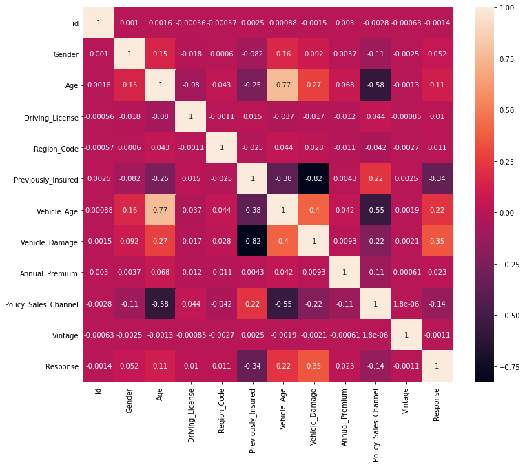
Feature Correlation using Pearson Correlation co-efficient the closer to 1 the better we can deduce from the plot that Vehicle_Damage is the most correlated feature with our target variable(Response).
Modelling Part
Splitting the data
X = df.drop(["Response", 'id'], axis=1)
y = df["Response"]
# spliting the data to train and validation set
# train and test data
X_train, X_test, y_train, y_test = train_test_split(X, y, random_state=101,stratify=y)
# shape of the data of train and validation set
print('Shape of the X_train {}'.format(X_train.shape))
print('Shape of the y_train {}'.format(y_train.shape))
print('Shape of the X_test {}'.format(X_test.shape))
print('Shape of the y_test {}'.format(y_test.shape))
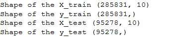
The shape of our data on train and validation. we will be using Lightgbm Algorithm to build our model.
Using Lightgbm Algorithm
    params = {}
    params["objective"] = "binary"
    params['metric'] = 'auc'
    params["max_depth"] = -1
    params["num_leaves"] = 10
    params["min_data_in_leaf"] = 20
    params["learning_rate"] = 0.03
    params["bagging_fraction"] = 0.9
    params["feature_fraction"] = 0.35
    params["feature_fraction_seed"] = 20
    params["bagging_freq"] = 10
    params["bagging_seed"] = 30
    params["'min_child_weight'"] = 0.09
    params["lambda_l1"] = 0.01
    params["verbosity"] = -1
from lightgbm import LGBMClassifier # intializing the model
model = LGBMClassifier(**params)
# fitting the model
model.fit(X_train, y_train)
Checking our model performance using ROC_AUC score.
def model_auc(model):
    train_auc = roc_auc_score(y_train, model.predict_proba(X_train)[:, 1])
    val_auc = roc_auc_score(y_test, model.predict_proba(X_test)[:, 1])
    print(f'Train AUC: {train_auc}, Val Auc: {val_auc}')
# model performance
model_auc(model)
# predicting the likelihood for the validation set
y_pred = model.predict_proba(X_test)[:, 1]
# checking the roc_auc_curve
print('AUC score of the model is {}'.format(roc_auc_score(y_test, y_pred)))
# the visualization of roc_auc score
plot_roc_curve(model, X_test, y_test)
.png)
.png)
The above plot shows our roc_auc score and plot.
Feature Importance of the model
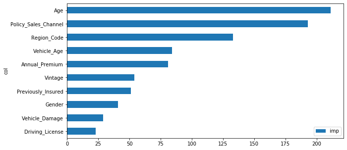
Global feature importance quantifies the relative importance of each feature in the test dataset as a whole. It provides a general comparison of the extent to which each feature in the dataset influences prediction.
The above plot shows the weight and values each feature has contributed to the Response may be a customer will be interested or not interested in the Vehicle Insurance. from the above features so many questions will arise for the businesses.
- The features at the top 5 which one is more contributing to the class 0 or class 1
- The Decision needs to be more transparent
Explainable AI(Using Lime and Shap)
Local feature importance measures the influence of each feature value for a specific individual prediction.
Lime
This is a model agnostic approach, which means it is applicable to any model in order to produce explanations for predictions.
Using Lime to make decision
from lime.lime_tabular import LimeTabularExplainer
class_names = [0, 1]
#instantiate the explanations for the data set
limeexplainer = LimeTabularExplainer(X_test.values, class_names=class_names, feature_names = X_test.columns, discretize_continuous = True)
idx=0 # the rows of the dataset
explainable_exp = limeexplainer.explain_instance(X_test.values[idx], model.predict_proba, num_features=3, labels=class_names)
explainable_exp.show_in_notebook(show_table=True, show_all=False)
.png)
.png)
We can see the Top 3 features and the actual class our customer at index 0 belongs. Lime makes it more explainable to us in terms of the weight and values of an attribute that makes the customer interested in the Vehicle Insurance Policy.
SHAPLY VALUES
It has optimized functions for interpreting tree-based models and a model agnostic explainer function for interpreting any black-box model for which the predictions are known.
explainer = shap.TreeExplainer(model)
expected_value = explainer.expected_value
if isinstance(expected_value, list):
    expected_value = expected_value[1]
print(f"Explainer Expected Value: {expected_value}")
idx = 100 # row selected for fast runtime
select = range(idx)
features = X_test.iloc[select]
feature_display = X.loc[features.index]
import warnings
warnings.simplefilter(action='ignore', category=FutureWarning)
with warnings.catch_warnings():
    warnings.simplefilter('ignore')
    shap_values = explainer.shap_values(features)[1]
    shap_interaction_values = explainer.shap_interaction_values(features)
if isinstance(shap_interaction_values, list):
    shap_interaction_values = shap_interaction_values[1]
.png)
Summary Plot(more consistent and trustworthy than feature importance)
.png)
From the above summary, the plot is different from Global feature importance but similar to the top 3 features with the LIME feature importance.
Summary Plot(to check features shift the decision positively or negatively)
.png)
From the plot we can deduce that when Previously_Insured is 0 and Vehicle_Damage is 1 it’s contributing more to the positive class(1). We can also see from the Driving_License Feature a particular customer is behaving, which is helpful for model debugging.
Dependency Plot(One-way Plot checking 100 customer’s behavior)
shap.dependence_plot(ind='Age', interaction_index='Age',
                    shap_values=shap_values, features=X_test[:idx],
                    display_features=feature_display)
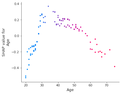
The ages from 20-35 years from are behaving to the model negatively and 40-50 years behaving positively to the model of the 100 selected customers.
Two Dependency Plot
shap.dependence_plot(ind='Age', interaction_index='Previously_Insured',
                    shap_values=shap_values, features=X_test[:idx],
                    display_features=feature_display)
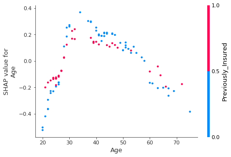
We observe the 2-way interaction of the Age separated by previously insured value with either 0 or 1.
Force Plot Individually
shap.initjs() # run to show the plot
shap.force_plot(explainer.expected_value, shap_values=shap_values[0,:], features=feature_display.iloc[0,:])
.png)
Showing the features moving the decision to a positive value for the customer at index 0. it shows the base prediction of the customer is -0.92 and we can deduce that Vehicle_Damage = 1, Previously_Insured = 0, Age = 46, and Policy_Channel = 26, are moving the customer to a positive value.
Multiple Force Plot
shap.force_plot(explainer.expected_value, shap_values, feature_display)
.png)
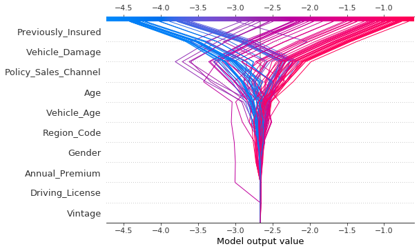
Decision Plot
shap.decision_plot(expected_value, shap_values, features)
Conclusion
Explainable AI(Lime and Shap) can help in making our black-box model more interpretable to the businesses. Explainable AI can be used with any Algorithm(Logistic or Linear Regression, Decision Tree, and others).


