An end-to-end comprehensive guide for PCA
Introduction
One of the most sought-after and equally confounding methods in Machine Learning is Principal Component Analysis (PCA). No matter how much we would want to build our models without dealing with the complexities of PCA we would not be able to stay away from it for long. The beauty of PCA lies in its utility. It involves concepts such as subset, largest eigenvalue, eigenvectors of the covariance matrix, cov, scatter plot, and various machine learning algorithms.
In this article, firstly we will intuitively understand what is PCA, how it is done, its purpose. Post which we will dive deep into the mathematics behind PCA: linear algebraic operations, the mechanics of PCA, its implications, and applications.
.jpg)
Learning Outcomes
- Gain a solid understanding of Principal Component Analysis (PCA).
- Learn about the applications of PCA in real-world data analysis.
- Understand how to conduct PCA on high-dimensional datasets.
- Learn how to improve the Signal to Noise Ratio (SNR) using PCA.
- Apply dimensionality reduction techniques for efficient data visualization and preprocessing.
This article was published as a part of the Data Science Blogathon.
Table of contents
- Introduction
- Introduction
- Signal to Noise Ratio (SNR)
- Curse of Dimensionality
- Step by Step Approach to conduct PCA
- Improving SNR via PCA
- Linear Algebraic Operations for PCA
- Example of Singular Value Decomposition
- Dimensionality Reduction
- Variable Reduction
- Can PCA be used for every kind of data?
- Final thoughts
Introduction
Let’s begin by discussing your preferred radio station. Personally, I enjoy tuning in to 104.8 FM, especially for its lineup of love songs. Now, when we set our dial to the 104.8 frequency, we’re greeted with the station we desire. But here’s an interesting observation: even if we slightly adjust the frequency, like tuning to 105 or 104.5, we can still pick up the radio station. However, as we move further away from the 104.8 frequency, something peculiar begins to occur. Allow me to illustrate this concept more explicitly.
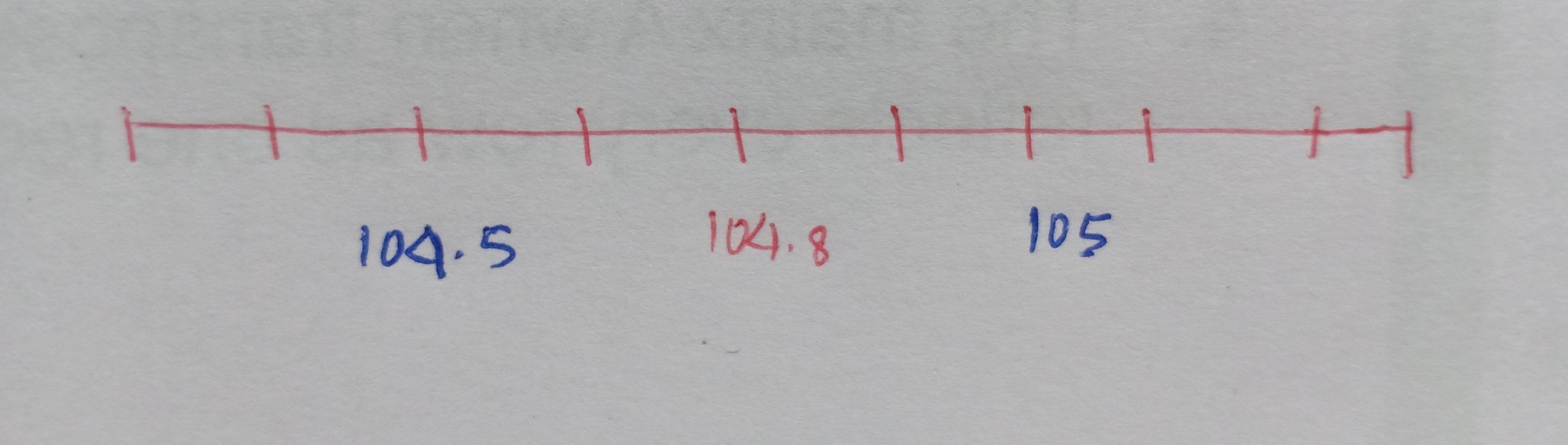
The x-axis represents the FM frequencies and we have 104.8 as our desired radio channel pitch.
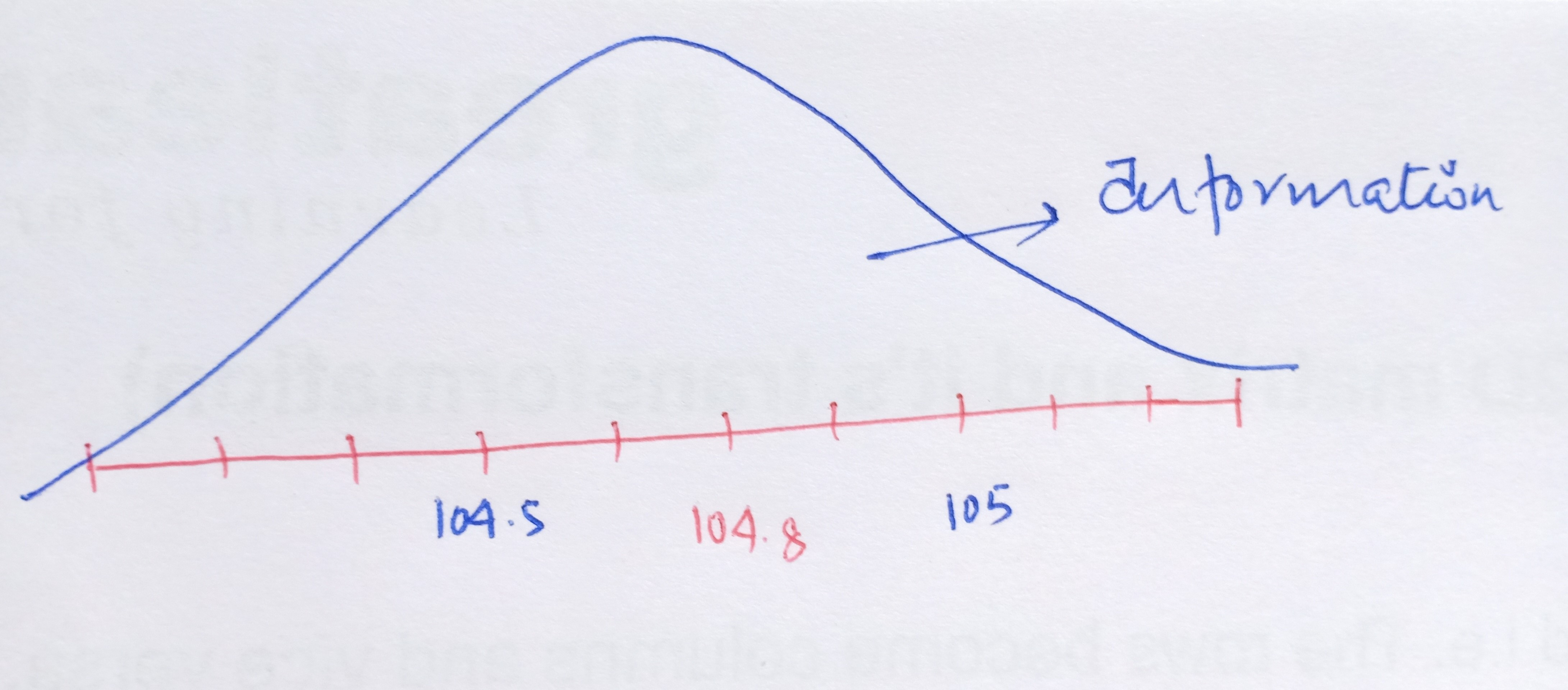
Now, as we move further away from the required FM frequency either on the higher side or on the lower side, we start to get unwanted signals i.e. the broadcast of the radio gets jumbled up with the noise. In other words, we get the maximum volume or the amplitude of our needed station at that particular frequency of 104.8 but the volume of the channel drops as we diverge from 104.8. This leads us to the concept of noise and signal.
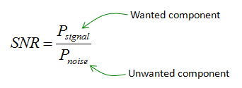
In Statistics, the signal of interest to us or the information present is stored in the spread (or the variance) of the data. In our example, the frequencies are the information that we need. This is also known as the Signal to Noise Ratio.
Signal to Noise Ratio (SNR)
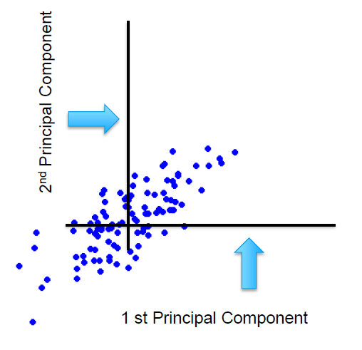
We have a mathematical space consisting of two dimensions x1 and x2 and the data between these two dimensions is scattered as shown below.
When we look at the space from the point of view of x1 only then the amount of spread ranges between x1min and x2 max, that is the information content captured by x1. And, seeing the data from x2 the signal or amount of spread expressed by x2 dimension ranges from x2min and x2 max.
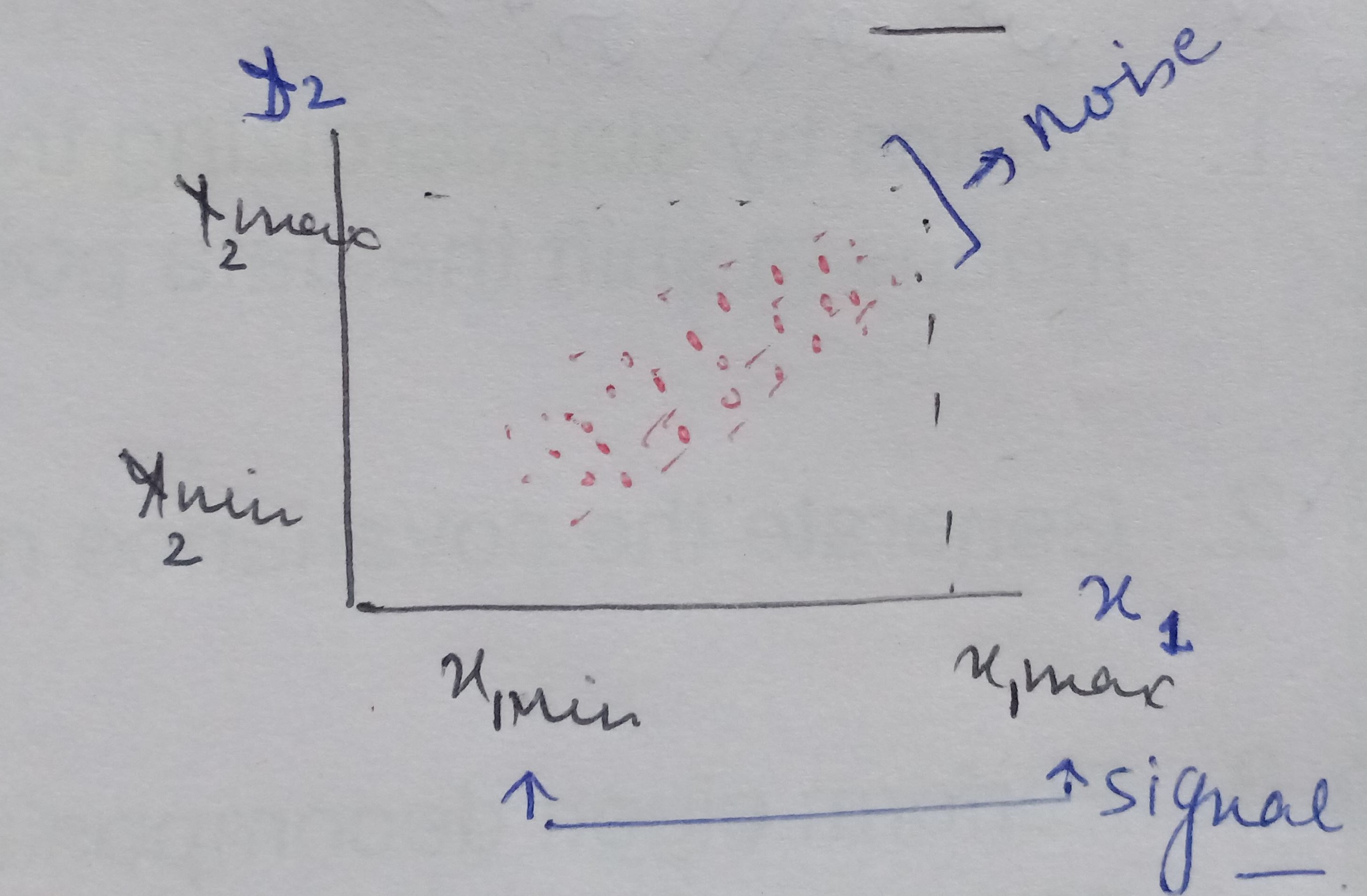
On analyzing this data together by considering both x1and x2, we see there is a larger spread containing information about how x1 and x2 influence each other. When seeing the data from x1 ‘s point of view then the data present in the other dimension that is the spread or the vertical lift in the data points is only noise for x1 cause x1 is unable to explain this variation. Similarly, the vertical lift in the data points is also noise from x2’s view as x2 also cannot explain this spread either.
Therefore, on putting the data points present in both the dimensions together we see there is covariance present in the mathematical space that shows that x1 and x2 influence each other.
Hence, the signal is all the valid values for a variable ranging between its respective min and max values and the noise represented by the spread of the data points across the best fit line. This unexplained variation in the data is due to random factors.
The objective of PCA is to maximize or increase this signal content and reduce the noise content in the data.
Now, shifting the gears towards understanding the other purpose of PCA.
Curse of Dimensionality
When building a model with Y as the target variable and this model takes two variables as predictors x1 and x2 and represent it as:
Y = f(X1, X2)
In this case, the model which is f, predicts the relationship between the independent variables x1 and x2 and the dependent variable Y. On building this model using any of the algorithms available, we are essentially feeding x1 and x2 as the inputs to the algorithm. What this means is that this algorithm gets its input from the information content present in the x1 variable and the information content present in the x2 variable as the two parameters.
All the algorithms assume that these parameters which make the mathematical two-dimensional space along with the target variable are independent of each other, that is x1 and x2 do not have an influence on each other. Y is strongly dependent on X1 and X2 respectively. This assumption of X1 and X2 being independent of each other is often violated in reality.
When X1 and X2 are dependent on each other, then these variables end up interacting with each other. In other words, there is a correlation present amongst them. When two independent variables are very strongly interacting with each other, that is the correlation coefficient is close to 1 then we are providing the same information to the algorithm in two dimensions, which is nothing but redundancy. This unnecessarily increases the dimensionality of the features of the mathematical space. When we have too many dimensions more than required then we are exposing ourselves to the Curse of Dimensionality.
The impact of having more dimensions in the model, which is nothing but having multicollinearity in the data can lead to overfitting, and this exposes the model to have variance errors, that is the model may fail to perform or predict for new unseen data.
PCA also helps to reduce this dependency or the redundancy between the independent dimensions.
We shall see in detail later how PCA helps to reduce this redundancy in the dimensions. Having seen what PCA is, its purpose let’s now explore how PCA works along with the mathematics involved in it.
Step by Step Approach to conduct PCA
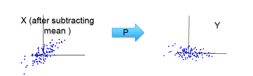
What PCA does is, it essentially rotates the coordinate axes, in a such way that axis captures almost all the information content or the variance. The clip below visually depicts it. We’ll go step by step to see how this is achieved.
We saw above that the two independent parameters X1 and X2 are fed into the model. In Python implementation, we shall do it using model.fit(x1, x2). As we know by now, that the model is only capturing the individual respective information available in the predictors and not the joint spread which is far richer as it tells how these two variables vary together. This with each other is captured in the model till yet and the covariance
The aim of PCA is to capture this covariance information and supply it to the algorithm to build the model. We shall look into the steps involved in the process of PCA.
The workings and implementation of PCA can be accessed from my Github repository.
Step1: Standardizing the independent variables
When we apply Z-score to the data, then we are essentially centering the data points to the origin. What do we mean by centering the data?
From the above FM frequencies chart, let’s say 104.8 is the central value i.e the average or the mean value represented by x-bar and other frequencies are xi values. On converting these xi values to Z-score, where Z = (xi – x bar)/standard deviation
Take any xi value, the distance in the units of standard deviation that is how many standard deviations away this xi value is from the central value or the average is, what is represented by the Z-score of this xi point.
When the xi is more than the average then this calculated distance in terms of standard deviation or in other words, the Z-score will be positive and the Z-score will be negative when the xis are less than the x-bar. As the Z-score becomes positive to negative when crossing over the central value then substituting this xi = x-bar in the Z-score formula = (xi – x bar)/standard deviation, the numerator becomes zero.
In short, the process of standardizing is we are taking all the data points and shifting the average value of frequencies from 104.8 to make it zero. This means that data on all the dimensions are subtracted from their means to shift the data points to the origin.
Post this standardization, all the frequencies (data points) that were on the higher side of the average of 104.8 became positive values and all the frequencies that were on the lower side of the average of 104.8 became negative values. This is known as centering.
Step 2: Generating the covariance or correlation matrix for all dimensions
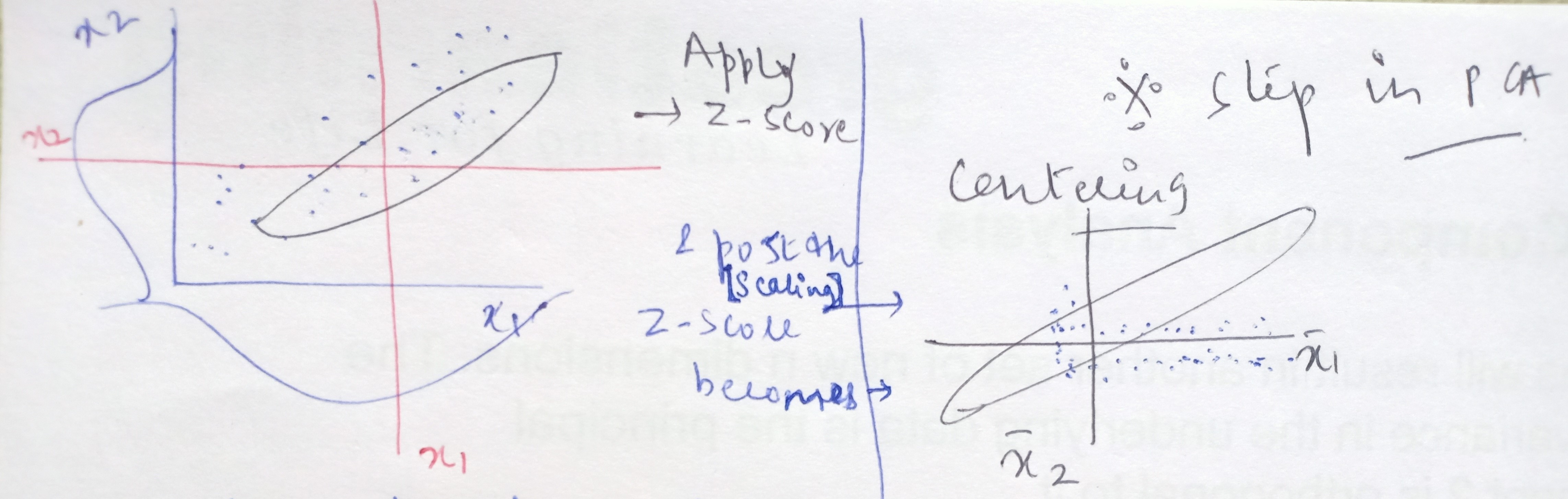
In the next step, we capture covariance information between all the dimensions put together. In the original two dimensional space, the data looks like below with x1-bar and x2-bar as the respective averages and have covariances between x1 and x2.
When we standardize the data points then what happens is that the central values become the dimensions and the data is scattered around it. On this conversion of xis to Z-scores, the xi values get shifted from the original space to a new space where the data gets centered and all the axes are the x1 bar, x2 bar, x3 bar, and so on.
In this new mathematical space, we find the covariance between x1 and x2 and represent it in the form of a matrix and obtain something like below:
This matrix is the numerical representation of how much information is contained between the two-dimensional space of X1 and X2.
In the matrix, the elements on the diagonals are the variance or spread of x1 with itself and of x2 with itself implying how much information is contained within the variable itself. Hence, the diagonals will almost always be close to one as it shows how the variable behaves with self.
The degree of signal or information is indicated by the off-diagonal elements. These indicate the correlation between x1 and x2 that is how these two interact or vary with each other. A positive correlation suggests a positively linear relationship and the negative correlation value represents a negative linear relationship. It is highly imperative to use this newly found information as an input for building our model.
Step 3: Eigen Decomposition
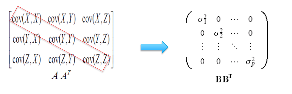
The process of eigendecomposition transforms the original covariance matrix between X1 and X2 into another matrix that looks like the below matrix.
In this new matrix, the diagonals are one and off-the-diagonal elements become close to zero. This matrix represents that mathematical space where there is no information content at all. All the information content is on the axis meaning the axis has observed all the information content and the new mathematical space is now empty.
During this process, we get two outputs as below:
-
Eigen Vectors: These are the new dimensions of the new mathematical space, and
-
Eigenvalues: This is the information content of each one of these eigenvectors. It is the spread or the variance of the data on each of the eigenvectors.
We shall look at the meaning and the mathematics of these outputs of eigenvectors and the eigenvalues and how the axes absorb all the signals in detail below.
Step 4: Sort the Eigenvectors corresponding to their respective eigenvalues
Principal Component Covariance Matrix
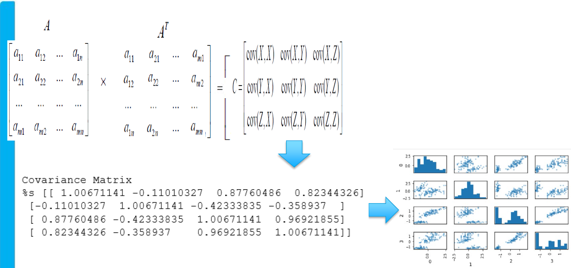
Mathematically, we obtain the covariance matrix from a given matrix by multiplying the matrix with its transpose form. The covariance matrix is nothing but the numerical form of the pair plot that we get from sns.pairplot().
Below is an example of associating the matrix and the pair plot. In the pair plot, we can see that there is some correlation between the two variables, and that relationship is represented in the numerical form in this covariance matrix. Hence, this matrix reflects how much information is there in the mathematical space and the pair plot is a graphical depiction of the same.
The diagonals in the pair plot show how the variables behave with themselves and the off-diagonal shows the relationship between the two variables in the same manner as it was for the covariance matrix. As we know by now that this information off-the-diagonal is not yet fed to the model and our hypothesis is once we send these off-diagonal signals also to the model then the model performance will be better and so would reflect in the production.
Improving SNR via PCA
The first step to conduct PCA was to center our data which was done by standardizing only the independent variables. We had subtracted the average values from the respective xis on each of the dimensions i.e. had converted all the dimensions into their respective Z-scores and this obtaining of Z-scores centers our data.
For two-dimensional data, the above visual illustrates that earlier the axes were the respective x-bars and now these are the new dimensions. The data is still oriented in the same way as was in the original space only thing is it has become centered now.
This information is converted into the covariance matrix. On this covariance matrix, we apply the eigenfunction, which is a linear algebra function. The dimensions are transformed using this algebra into a new set of dimensions.
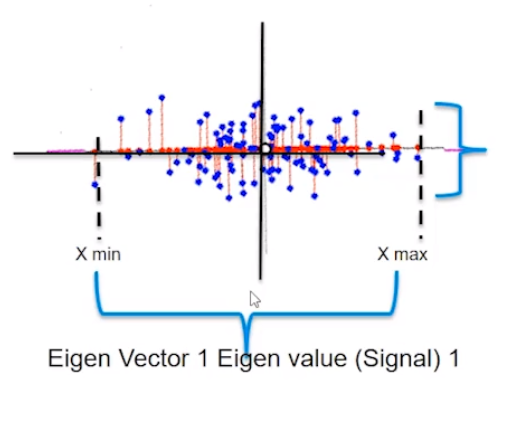
On applying the eigenfunction, what conceptually happens is that mathematical space is rotated. The transformation is a rotation of axes in a mathematical space and identifies two new dimensions that are called eigenvectors: E1 and E2.
These eigenvectors are nothing but the principal components. These are the directions in the original mathematical space where the maximum spread is captured. The spread is the signal or information content.
The amount of spread each eigenvector captures or in other words the variance across in each of the eigenvectors is expressed in the eigenvalues. So, in our two-dimensional space, the eigenvector E1 has an associated eigenvalue, ev1, and eigenvector E2 has another associated eigenvalue, ev2.
In the original space, we had two dimensions x1 and x2, and hence will get two eigenvectors. The number of eigenvectors or principal components (or the new dimensions) will always be equal to the number of dimensions in the original space. Each of these eigenvectors will be orthogonal meaning will be at 90 degrees to each other. It is beyond our imagination and the scope of the article to visually depict how the components are at 90 degrees to each other for the higher dimensional space.
In the graph below, we can see that the eigenvectors, which are represented on the axis, contain all the information and there are no data points (or there are zero signals) in the mathematical space other than the axes. All the information is captured in the eigenvector E1 or E2.
Once we construct the covariance matrix of these eigenvectors, we get a matrix-like below.
This shows that the diagonal elements having a value of 1, explains all the information present in the data, and the off-diagonal elements, theoretically with the value of zero depict that there is no signal or information content. In reality, the off-diagonal elements will be close to zero and not exactly zero.
The original data points are now represented by the red dots on the new dimensions.
Now, let’s get our hands dirty by digging into the mathematics behind PCA.
Linear Algebraic Operations for PCA
PCA is basically one type of Singular Value Decomposition (SVD). In simpler terms, what it means that we are breaking or decomposing a larger value (i.e. a singular value) into smaller values. With reference to our context, we had divided our covariance matrix (the larger singular value) which was obtained post scaling of the independent variables into two outputs above the eigenvectors (into smaller values) and got their respective eigenvalues.
That’s pretty much what SVD is however, mathematically it can be a daunting task. For our purpose here, we will look into the bare minimum mathematical operations required to understand the workings of PCA.
Any matrix let’s say, A of dimension m * n, where m is the number of rows and n is the number of columns:
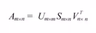
Can be further decomposed into the following way:
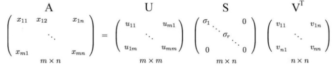
where U and V as the orthogonal matrices with orthonormal eigenvectors chosen from AAᵀ and AᵀA respectively. S is a diagonal matrix with r elements equal to the root of the positive eigenvalues of AAᵀ or Aᵀ A (both the matrices have the same positive eigenvalues anyway)
The diagonal elements are composed of singular values. In short, S is a diagonal matrix with positive values and is called a Singular matrix.
Don’t worry we shall look at what these greek terms do with an example below. Firstly, we need to understand the following two properties of the matrices:
-
Orthogonal Matrix:
Here, U and V are orthogonal matrices. This means that when we take the cross product (or, in mathematical terms the dot product) of the U and V then that resultant is zero.
U*V = 0 : Orthogonal Vectors
In statistical terms, two matrices are orthogonal means these matrices are independent of each other.
-
Orthonormal Matrix:
When a matrix is orthonormal it means that: a) the matrices are orthogonal and b) the determinant (that value which helps us to capture important information about the matrix in a just single number) is 1.
|U|=1, |V|=1 and U*V=0 : Orthonormal vectors
In case, we have a square matrix, meaning having the same number of rows and columns then it can be divided into smaller value in the following manner:
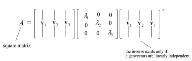
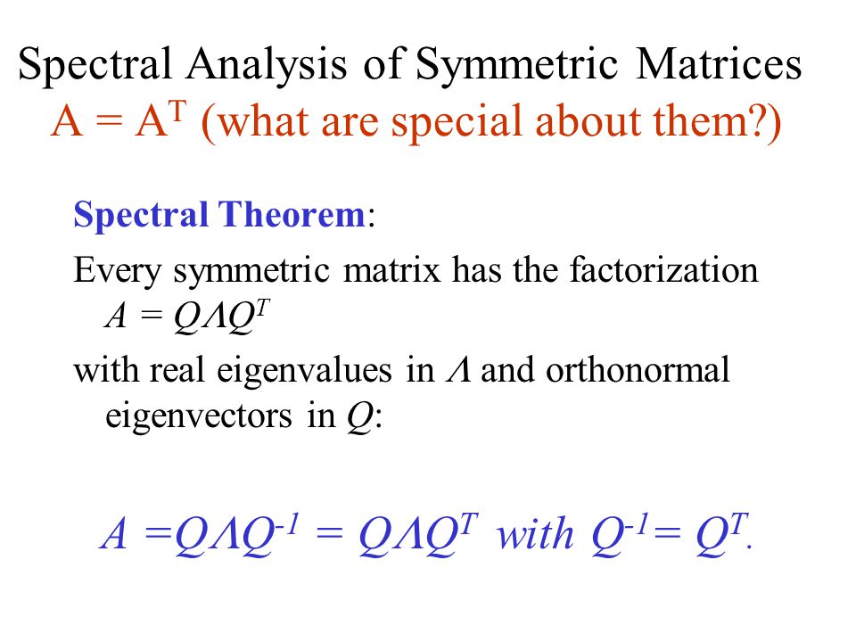
Mathematically, what the eigenvectors and eigenvalues mean is based on the Spectral Theorem. The theorem as follows (we shall not drive or prove the theorem here) :

Source: slideplayer
Example of Singular Value Decomposition
Let’s see the background calculation of this. Say A is the correlation matrix as below:
Step 1: How do we calculate the matrices U and V? We obtain it by taking the transpose of matrix A.
Step 2: The resultants that we get using the matrix A and its Transpose matrix Aᵀ is:
U = A* Aᵀ, and
V = Aᵀ * A

Step 3: Take the U = A* Aᵀ and calculate the eigenvectors and their associated eigenvalues.
Step 4: Using the output that is the eigenvector obtained in step 3, we calculate the Singular values matrix, S. This singular value is the square root of the eigenvectors.
Step 5: Multiplying the three matrices: U, S, and V as shown below, the end matrix is the same as the original matrix A.
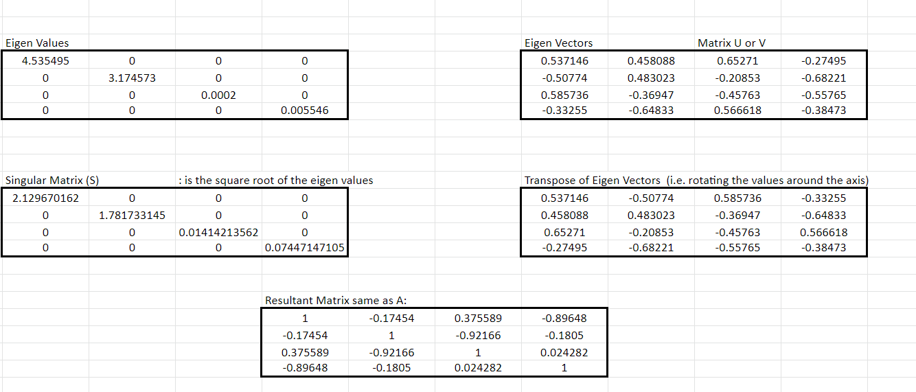
We can see that the S matrix represents something similar to the matrix that we obtained from performing PCA. It shows that the values on the diagonal are the information or the signal as all the axes absorb all the information and the off-diagonal elements do not have any signal content.
Dimensionality Reduction
The secondary objective of PCA is dimensionality reduction. How can we reduce the dimensions without losing the information content present in the variables? Whenever we remove any of the features we are losing the signal or the information available in the data.
As seen above, when there is a stronger linear relationship between X1 and X2 variables, then the more redundant the dimensions become. We can choose to drop any of the dimensions, say if we remove the X2 variable then we are at a loss of information as the signal available in X2 is not present in the X1 variable and vice-versa in case we choose to keep X2 and drop X1 variable then there is some loss of information again as X2 will not contain the information present in the X1 variable.
Hence, when there is a strong interaction between dimensions of the data then instead of dropping any one of the variables and losing information we can make use of PCA and create one composite dimension out of the two original dimensions and drop both the original features.
What will PCA do? PCA creates the first principal component, PC1, and the second principal component, PC2 is 90 degrees to the first component.
Both these components absorb all the covariances present in the mathematical space. We can then drop the original dimensions X1 and X2 and build our model using only these principal components PC1 and PC2. The reason we can the build model only using the components is that as had seen there is no covariance present among the components ie the off-diagonal information content is zero in the new mathematical space (though in reality, the covariance is close to zero), and hence absorbs all the information.
However, it still doesn’t help us to drop the dimensions. The number of dimensions is still two as equal to the original number of dimensions. But we can do something here, we can find out the cumulative information across all the principal components put together.
The first principal component, PC1 will always contain the maximum i.e. the major part of the covariance information, and will have the highest eigenvalue indicating this component captures the maximum information. We can follow the below steps to perform the dimensionality reduction:
-
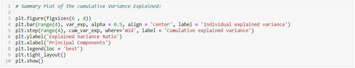
Arrange all the principal components (i.e. the eigenvectors) along with their corresponding eigenvalues in descending order and make a summary plot as shown below.
-
Based on this summary plot, we can drop those components that do not have any significant contribution to the total eigenvalues.
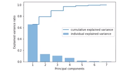
How do we read the above plot? The graph tells the first principal component captures about 64% of the information present in the original mathematical space i.e. explains ~ 64% of the variation in the data. On taking the first two components together, the total explained variation is close to 78% and when taking the first three components, then the cumulative explained variation is ~ 90% and ~ 99% of the variation is captured by the first four principal components. The other principal components 5, 6, and 7 are insignificant as they do not make any contribution suggesting these are not explaining much information and hence can be dropped.
This way when starting to build the model with seven dimensions, we can drop the three insignificant principal components and build the model with the remaining four components. Using this analysis, we reduce the seven-dimensional mathematical space to four-dimensional mathematical space and lose only a few percentage points of the data. Hence, we can reduce the dimensionality in the data without losing much information.
We can also apply another method known as Linear Discriminant Analysis (LDA) to reduce the dimensionality, though this method is beyond the scope of the article.
Variable Reduction
Now, apart from increasing the Signal to Noise Ratio (SNR) and reducing the dimensionality, there’s another objective of PCA. It is to reduce the variables.
How it is done is by grouping the variables based on similarity (i.e. those variables which have high correlation) are grouped together. This goal of PCA is helpful in business problems where it is required to classify the data into n-number of classes and the n is not predefined, in short in segmentation problems.
To see and understand how this works, we shall approach the mechanics of PCA in a different manner than what we had seen above. The steps involved in calculating the PCAs are the same as described above, what differs is the conceptual underlying story to arrive at the PCA.
Let’s say we are building a model having ten predictors Xs with target variable Y and the original equation for the model based on the linear regression algorithm is like below:
Y = B1X1+ B2X2+… + BnXn + C
Where Xs are the dimensions of the data and are not independent of each other
We are applying PCA to drive new features or known as the components based on these original ten X variables. PCAs are also calculated as the linear combinations of the original variables (Xs) to generate the axes, (also known as the principal components) and having weights Wi.
Now, the regression-based on PC, or referred to as Principal Component Regression has the following linear equation:
Y = W1* PC1 + W2* PC2+… + W10 * PC10 +C
Where, the PCs: PC1, PC2….are independent of each other and the correlation amongst these derived features (PC1…. PC10) are zero. Hence, PCs are the functions of Xs.
In interpreting the principal components, it is useful to know the correlations of the original variables with the principal components. We are deriving the new dimensions (or components) in such a way that the derived variables are linearly independent of each other and hence, multicollinearity present in the data is taken care of.
The reason why the derived dimensions are independent of each other is because of the orthogonality condition of the matrices we saw above that stated the cross product of U and V is zero (hence, implying correlation is zero between these two matrices.)
Now, shifting the gears to understand how are the PCs are derived and how the weights are estimated, and most importantly what do they signify and how it helps to reduce the variables.
How are the PC dimensions derived?
To apply PCA, we take the standardized (Z-scores) of each of the variables say it’s denoted by Z_X1, Z_X2….Z_X10 and in the second step we obtain the correlation matrix of these Z-scores values, which is nothing but is a square Matrix and we had seen above that any matrix can be decomposed using the singular value decomposition.
Based on these standardized Z-scores and the coefficients (which is the betas), we get the PC1, PC2… PC10 dimensions. Each of these derived components has a respective following equation:
B11* Z_X1 + B12* Z_X2 +… + B110* Z_X10
B21* Z_X1 + B22* Z_X2 +… + B210* Z_X10
….
B101* Z_X1 + B102* Z_X2 +… + B1010* Z_X10
How are these weights or the betas estimated?
The betas get estimated such that these satisfy the following criteria:
Corr(Pci, PCj) ~0
Var(PC1) + Var(PC2) +… Var(PC10) = 10
Var(PC1) > Var(PC2) >… Var(PC10)
The eigenvectors of a square matrix of the correlation matrix is the same as that of the betas ( or coefficients) calculated in the PC Regression and hence, these two are related. Also, as know by now that each of the PCs or the principal components have their associated Eigenvalues, which are the variance or the spread explaining the information content present in that dimension.
In summary, what we have from applying the PCA process is:
i) PC1, PC2,….PC10 is derived and independent features from X1, X2…X10
As seen above, if the original variables are 10 then it will create 10 new dimensions.
ii) Corr between the PCs: Corr(Pci, PCj) ~0 , where i and j are different
iii) Var(X1) + Var(X2) + Var(X3) …+ Var(X10) = Var(PC1) + Var(PC2) +… Var(PC10)
This implies that the total variation explained by all the Xs is also explained by the principal components. If each variable explains or contributes 1 variation then the total variation explained by all the variables is 10, and
iv) Var(PC1) > Var(PC2) >… Var(PC10), indicating that PC1 the first component explains the maximum variance followed by the variation explained by PC2 and so on.
How do we reduce the Variables using PCA?
Firstly, we calculate the correlation between the standardized Z-score value of each of the variables with each of the principal components.
So, let’s say the first X variable has the Z-score of Z_X1 and PC1 is the first component, the correlation between these two is nothing but the betas i.e. B11.
Following in the linear equation for the first component:
PC1 = B11*Z_X1 + B12*Z_X2 +….. + B110*Z_X10
The betas are the correlation as these indirectly imply how much of X is contributing to the principal components. In the above equation, B11 implies how much of X1 is contributing to PC1.
As the Z_Xs are the standardized scores, meaning all the X variables are on the same scale, so now what we can do is we can compare the betas (coefficients) of each of the scores.
If B12 is the highest then can conclude that Z_X2 is having the maximum contribution (or the maximum impact) on the first component, PC1 and Z_X2 has a high correlation with PC1.
This concludes, the higher the betas (or the coefficients) tells which the Xs are having more impact on the PCs. Hence, based on these coefficients or the correlation computed between the standardized scores and the principal components, we can get the variables that have the maximum contribution.
Factor Loadings and How to choose the Variables?
The coefficients, or the calculated correlation between the standardized scores and the principal components, are also known as the factor loadings. The following table shows the loadings for five of the derived PC components for the original 10 X variables, where the Bis stands for the respective correlations.
Table 1 :
| PC1 | PC2 | PC3 | PC4 | PC5 | |
| Z_X1 | B11 = 0.12 | B21 | B31 | B41 | B51 |
| Z_X2 | B12 = 0.55 | B22 | B32 | B42 | B52 |
| Z_X3 | B13 = 0.25 | B23 | B33 | B43 | B53 |
| Z_X4 | B14 = 0.85 | B24 | B34 | B44 | B54 |
| Z_X5 | B15 = 0.17 | B25 | B35 | B45 | B55 |
| Z_X6 | B16 = -0.34 | B26 | B36 | B46 | B56 |
| Z_X7 | B17 = -0.11 | B27 | B37 | B47 | B57 |
| Z_X8 | B18 = 0.15 | B28 | B38 | B48 | B58 |
| Z_X9 | B19 = 0.74 | B29 | B39 | B49 | B59 |
| Z_X10 | B110 = 0.21 | B210 | B310 | B410 | B510 |
These loadings help us to choose which X variables are having more contribution to the PC variables. On analyzing the above table, we see:
-
The variables Z_X4, Z_X9, and Z_X2 for PC1 have higher correlation as compared to the others and hence, can conclude that these three variables are having the maximum contribution on PC1 (irrespective of the correlation is positive or negative).
-
Now, out of this can say that the correlation between Z_X4 and PC1 is higher than the correlation between Z_X9 and PC1.
-
So, when Z_X4 has a correlation with PC1; Z_X9 has a correlation with PC1 and Z_X2 has a correlation with PC1 then, we can also say that Z_X4, Z_X6, and Z_X2 have some correlation amongst themselves i.e. these variables are highly correlated with each other.
Hence, we can group these variables that have the maximum contribution on a respective principal component, PC and we get the following table.
Table 2:
| PC1 | X9 |
| X4 | |
| X2 | |
| PC2 | X3 |
| X5 | |
| X7 | |
| X10 | |
| PC3 | X1 |
| X2 | |
| X8 |
Table 2 tells us which variables contribute the maximum for that respective principal component. Based on the contribution of the variables, we have three components from the starting five principal components.
Now, on analyzing this table, we can make the following conclusions that if the variable X3 is contributing maximum on the principal component, PC2, then it will be less contributing on PC1 and PC3 because the PCs are independent of each other.
To conclude, once the loadings are grouped based on their contribution to the PCs then:
-
The X variables within each of the PCs are having some correlation amongst them (as said above in PC1 the variables X9, X4 and X2 are having some correlation among them and similarly other variables have correlation present within the respective components for PC2 and PC3)
-
Hence, based on the highest contributor of the variables to the PC we can select(or choose) any of the variables. For say for PC1, X9 is the highest contributor. In case, multicollinearity is an issue, then we can choose that variable that has the least correlation amongst all of the variables.
In case, there are more variables grouped together then can also choose two variables to represent that principal component.
A word of caution here, as in the above PC1, the three variables X9, X4, X2 have some correlation amongst them then this could lead to the issue of multicollinearity present in the PC components itself. It’s a challenge in the regression problems (i.e Linear and Logistic Regression) as these parametric techniques can lead to the issue of unstable estimation of the betas (or the coefficients) which is a serious consequence of multicollinearity. This can eventually lead to overfitting of the model as indicated by the insignificant betas (having p-value more than 0.05) that there are too many variables not contributing to the model accuracy.
However, in business problems based on Segmentation, this is not much of a problem.
Hence, the objective of PCA is to group the variable based on similarity (having high correlation) so the loadings which have a high contribution (correlation) are grouped together.
Can PCA be used for every kind of data?
PCA must be used in certain specific conditions only. The data must have a strong linear correlation between the independent variables. The spread in the data must look like either of the first two visuals and not like the last visual depicted in the graph below. In short, there must be high multicollinearity present in the data for PCA to be applied.
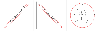
Source: gstatic.com
Final thoughts
The following illustration summarizes PCA very succinctly.
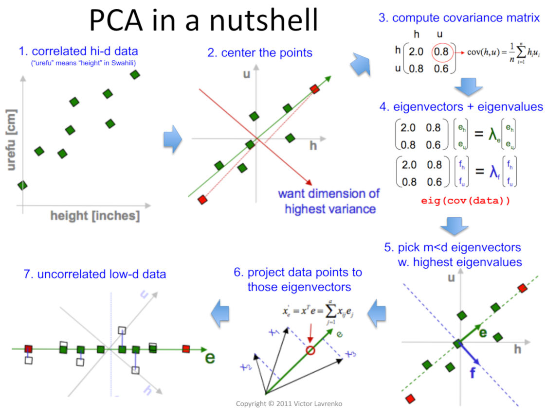
Source: Victor Lavrenko and Charles Sutton, 2011
The takeaway for us is that PCA feeds two birds with the one scone:
-
It increases the signal or the information content provided to the algorithm to build the model by transforming the existing dimensions to increase the Signal to Noise Ratio.
-
It helps to remove the dependency present in the data by eliminating the features that contain the same information as given by another attribute and the derived components are independent of each other.
Linkedin Profile: linkedin.com/in/neha-seth-69771111


Really love the explanations. Though I could grasp the concept on the first pass, I will have to re-read again to capture the all the math details. Thank you for your effort to put into the article.
Very informative article. Details are expressed in such a easy language. Anyone get useful knowledge.
It's very useful and helpful
Very very informative and technically an excellent work. Really like the way it was explained. My best wishes
Absolutely brilliant. Keep it up.
Excellent & very intelligent explanation of one of the most sought after topic of present time.Dr Sharad Lakhotia
Congrats ! It is really exhaustive and informative. Liked it. Keep it up !
A very elegant and elaborate elucidation.
A very comprehensive elaboration
This whole concept has been copied from the great learning tutoring session....i think this is quite against the guidelines of Great Learning Academy
The Best explaination of PCA I ever studied...👍