ML Interpretability using LIME in R
Overview
- Merely building the model is not enough without stakeholders not being to interpret the outputs of your model
- In this article, understand how to interpret your model using LIME in R
Introduction
I thought spending hours preprocessing the data is the most worthwhile thing in Data Science. That is what my misconception was, as a beginner. Now, I realize, that even more rewarding is being able to explain your predictions and model to a layman who does not understand much about machine learning or other jargon of the field.
Consider this scenario – your problem statement deals with predicting if a patient has cancer or not. Painstakingly, you obtain and clean the data, build a model on it, and after much effort, experimentation, and hyperparameter tuning, you arrive at an accuracy of over 90%. That’s great You walk up to a doctor and tell him that you can predict with 90% certainty that a patient has cancer or not.
However, one question the doctor asks that leaves you stumped – “How can I and the patient trust your prediction when each patient is different from the other and multiple parameters can decide between a malignant and a benign tumor?”
This is where model interpretability comes in – nowadays, there are multiple tools to help you explain your model and model predictions efficiently without getting into the nitty-gritty of the model’s cogs and wheels. These tools include SHAP, Eli5, LIME, etc. Today, we will be dealing with LIME.
In this article, I am going to explain LIME and how it makes interpreting your model easy in R.
What is LIME?
LIME stands for Local Interpretable Model-Agnostic Explanations. First introduced in 2016, the paper which proposed the LIME technique was aptly named “Why Should I Trust You?” Explaining the Predictions of Any Classifier by its authors, Marco Tulio Ribeiro, Sameer Singh, and Carlos Guestrin.
Built on this basic but crucial tenet of trust, the idea behind LIME is to answer the ‘why’ of each prediction and of the entire model. The creators of LIME outline four basic criteria for explanations that must be satisfied:
- The explanations for the predictions should be understandable, i.e. interpretable by the target demographic.
- We should be able to explain individual predictions. The authors call this local fidelity
- The method of explanation should be applicable to all models. This is termed by the authors as the explanation being model-agnostic
- Along with the individual predictions, the model should be explainable in its entirety, i.e. global perspective should be considered
How does LIME work?
Expanding more on how LIME works, the main assumption behind it is that every model works like a simple linear model at the local scale, i.e. at individual row-level data. The paper and the authors do not set out to prove this, but we can go by the intuition that at an individual level, we can fit this simple model on the row and that its prediction will be very close to our complex model’s prediction for that row. Interesting isn’t it?
Further, LIME extends this phenomenon by fitting such simple models around small changes in this individual row and then extracting the important features by comparing the simple model and the complex model’s predictions for that row.
LIME works both on tabular/structured data and on text data as well.
You can read more on how LIME works using Python here, we will be covering how it works using R.
So fire up your Notebooks or R studio, and let us get started!
Using LIME in R
Step 1: The first step is to install LIME and all the other libraries which we will need for this project. If you have already installed them, you can skip this and start with Step 2
install.packages('lime')
install.packages('MASS')
install.packages("randomForest")
install.packages('caret')
install.packages('e1071')
Step 2: Once you have installed these libraries, we will first import them:
library(lime)
library(MASS)
library(randomForest)
library(caret)
library(e1071)
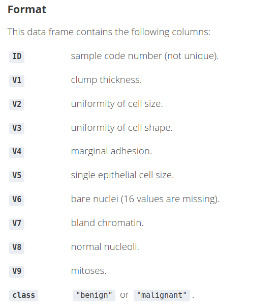
Since we took up the example of explaining the predictions of whether a patient has cancer or not, we will be using the biopsy dataset. This dataset contains information on 699 patients and their biopsies of breast cancer tumors.
Step 3: We will import this data and also have a look at the first few rows:
data(biopsy)
Step 4: Data Exploration
4.1) We will first remove the ID column since it is just an identifier and of no use to us
biopsy$ID <- NULL
4.2) Let us rename the rest of the columns so that while visualizing the explanations we have a clearer idea of the feature names as we understand the predictions using LIME.
names(biopsy) <- c('clump thickness', 'uniformity cell size',
'uniformity cell shape', 'marginal adhesion','single epithelial cell size',
'bare nuclei', 'bland chromatin', 'normal nucleoli', 'mitoses','class')
4.3) Next, we will check if there are any missing values. If so, we will first have to deal with them before proceeding any further.
sum(is.na(biopsy))
![]()
4.4) Now, here we have 2 options. We can either impute these values, or we can use the na.omit function to drop the rows containing missing values. We will be using the latter option since cleaning the data is beyond the scope of the article.
biopsy <- na.omit(biopsy)
sum(is.na(biopsy))
![]()
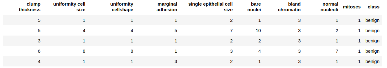
Finally, let us confirm our dataframe by looking at the first few rows:
head(biopsy, 5)
Step 5: We will divide the dataset into train and test. We will check the dimensions of the data
## 75% of the sample size

smp_size <- floor(0.75 * nrow(biopsy))

## set the seed to make your partition reproducible - similar to random state in Python
set.seed(123)
train_ind <- sample(seq_len(nrow(biopsy)), size = smp_size)

train_biopsy <- biopsy[train_ind, ]
test_biopsy <- biopsy[-train_ind, ]
Let us check the dimensions:
cat(dim(train_biopsy), dim(test_biopsy))
![]()
Thus, there are 512 rows in the train set and 171 rows in the test set.
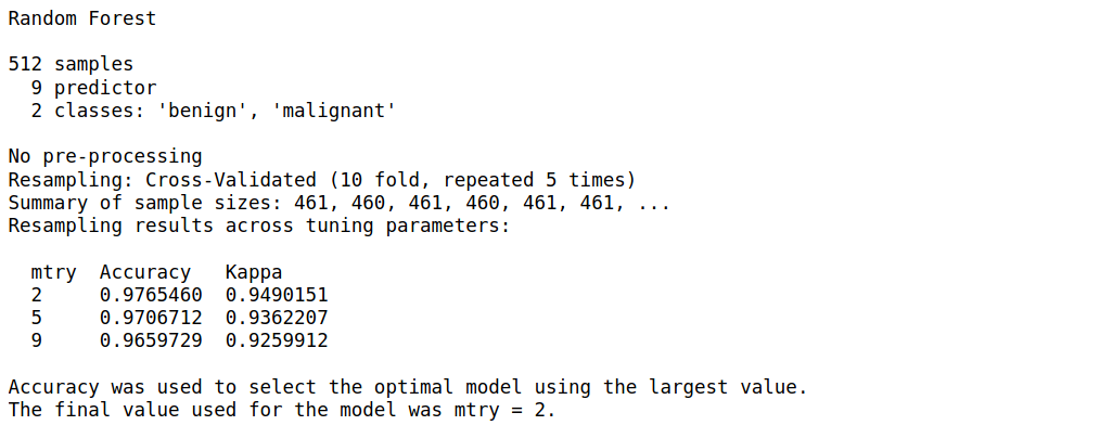
Step 6: We will be using a random forest model using the caret library. We will also not be performing any hyperparameter tuning, just a 10-fold CV repeated 5 times and a basic Random Forest model. So sit back, while we train and fit the model on our training set.
I encourage you to experiment with these parameters using other models as well
model_rf <- caret::train(class ~ ., data = train_biopsy,method = "rf", #random forest
trControl = trainControl(method = "repeatedcv", number = 10,repeats = 5, verboseIter = FALSE))
Let us view the summary of our model
model_rf
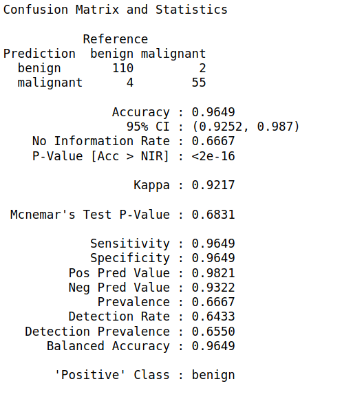
Step 7: We will now apply the predict function of this model on our test set and build a confusion matrix
biopsy_rf_pred <- predict(model_rf, test_biopsy)
confusionMatrix(biopsy_rf_pred, as.factor(test_biopsy$class))
Step 8: Now that we have our model, we will use LIME to create an explainer object. This object is associated with the rest of the LIME functions we will be using for viewing the explanations as well.
Just like we train the model and fit it on the data, we use the lime() function to train this explainer, and then new predictions are made using the explain() function
explainer <- lime(train_biopsy, model_rf)
Let us explain 5 new observations from the test set using only 5 of the features. Feel free to experiment with the n_features parameter. You can also pass
- the entire test set, or
- a single row of the test set
explanation <- explain(test_biopsy[15:20, ], explainer, n_labels = 1, n_features = 5)
The other parameters you can experiment with are:
- n_permutations: The number of permutations to use for each explanation.
- feature_select: The algorithm to use for selecting features. We can choose among
- “auto”: If
n_features <= 6use"forward_selection"else use"highest_weights" - “none”: Ignore
n_featuresand use all features. - “forward_selection”: Add one feature at a time until
n_featuresis reached, based on the quality of a ridge regression model. - “highest_weights”: Fit a ridge regression and select the
n_featureswith the highest absolute weight. - “lasso_path”: Fit a lasso model and choose the
n_featureswhose lars path converge to zero at the latest. - “tree”: Fit a tree to select
n_features(which needs to be a power of 2). It requires the last version ofXGBoost.
- dist_fun: The distance function to use. We will use this to compare our local model prediction for a row and the global model(random forest) prediction for that row. The default is Gower’s distance but we can also use euclidean, manhattan, etc.
- kernel_width: The distances of the predictions of individual permutations with the global predictions are calculated from above, and converted to a similarity score.
Step 9: Let us visualize this explanation for a better understanding:
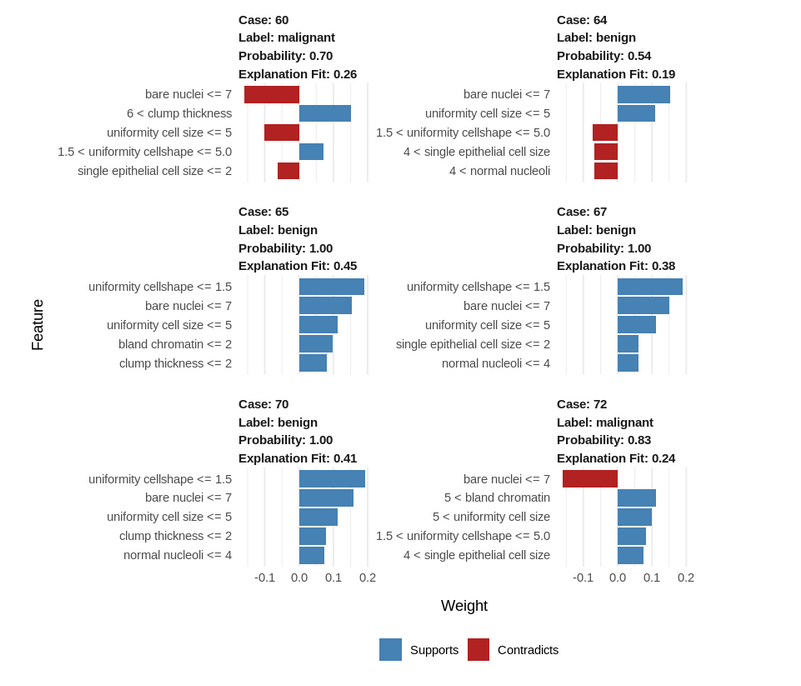
How to interpret and explain this result?
- Blue/Red color: Features that have positive correlations with the target are shown in blue, negatively correlated features are shown in red.
- Uniformity cell shape <=1.5: lower values positively correlate with a benign tumor.
- Bare nuclei <= 7: lower bare nuclei values negatively correlate with a malignant tumor.
- Cases 65, 67, and 70 are similar, while the benign case 64 has unusual parameters
- The uniformity of cell shape and the single epithelial cell size are unusual in this case.
- Despite these deviating values, the tumor is still benign, indicating that the other parameter values of this case compensate for this abnormality.
Let us visualize a single case as well with all the features:
explanation <- explain(test_biopsy[93, ], explainer, n_labels = 1, n_features = 10)
plot_features(explanation)
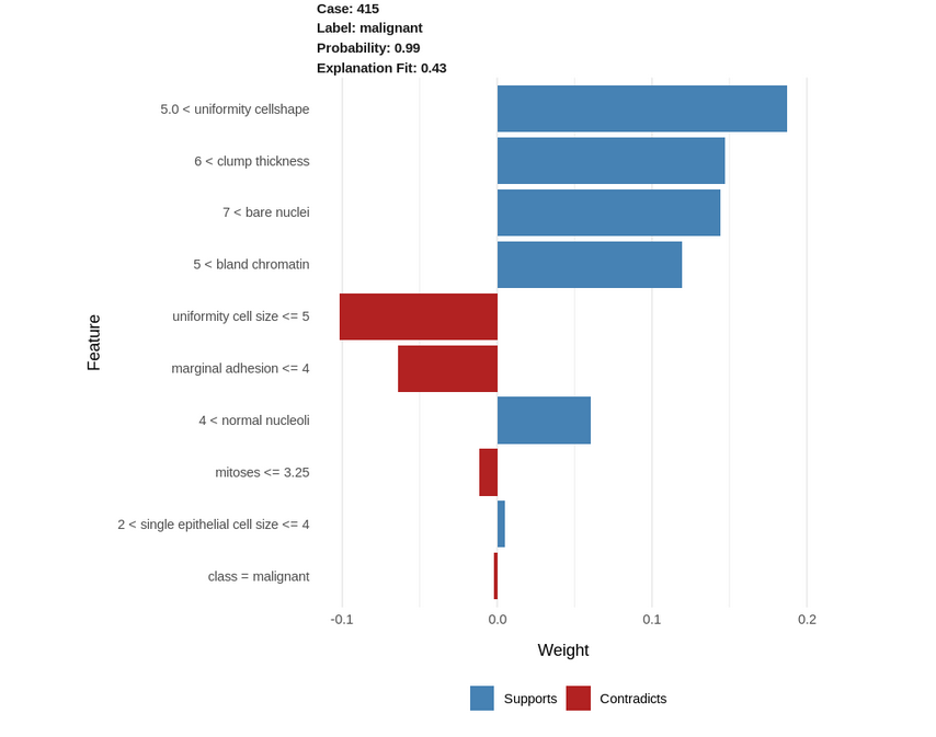
- Uniformity cellshape > 5.0: high values positively correlate with a malignant tumor(the higher this value, the more the chances of the tumor being malignant).
- Clump thickness > 6.0: high clump thickness values positively correlate with a malignant tumor.
- Similarly, bare nuclei > 7.0 and bland chromatin > 5.0 positively correlate with a malignant tumor.
- On the contrary, uniformity of cell size <= 5.0 and marginal adhesion <= 4: low values of these 2 parameters contribute negatively to the malignancy with a malignant tumor. Thus, the lower these values are, the lesser the chances of the tumor being malignant.
- Thus, from the above, we can conclude that higher values of the parameters would indicate that a tumor has more chances of being malignant.
We can confirm the above explanations by looking at the actual data in this row:

End Notes
Concluding, we explored LIME and how to use it to interpret the individual results of our model. These explanations make for better storytelling and help us to explain why certain predictions were made by the model to a person who might have domain expertise, but no technical know-how of model building. Moreover, using it is pretty much effortless and requires only a few lines of code after we have our final model.
However, this is not to say that LIME has no drawbacks. The LIME Cran package we have used is not a direct replication of the original Python implementation that we were presented with the paper and thus, does not support image data like its Python counterpart. Another drawback could be that the local model might not always be accurate.
I look forward to exploring more on LIME using different datasets and models, as well, exploring other techniques in R. Which tools have you used to interpret your model in R? Do share how you used them and your experiences with LIME below!


THANKS A LOT!!! Wonderful!!!
Hi @vlad, Thank you!
Any idea why this error appears? explainer % dplyr::select(-tj_year), xgb_fit_all_imp) # Explain the observations explanation Error in feature_distribution[[i]] : subscript out of bounds
Can I ask why the class = malignant appears in the plot when "class" is the label?
When i am writting the line : confusionMatrix(biopsy_rf_pred,as.factor(test_biopsy$class)) I'm getting this : [1] benign malignant (or 0-length row.names) Warning message: In Ops.factor(predictedScores, threshold) : ‘<’ not meaningful for factors Why this happening? Thanks in advance
When i'm writting the line: confusionMatrix(biopsy_rf_pred,as.factor(test_biopsy$class)) we get following: [1] benign malignant (or 0-length row.names) Warning message: In Ops.factor(predictedScores, threshold) : ‘<’ not meaningful for factors Why it's happening and how to rectify? Thanks in advance