Build Your First Linear Regression Machine Learning Model
This article was published as a part of the Data Science Blogathon.
Do you find AI and ML interesting?
Machine Learning and Artificial Intelligence are a few words in the current world that grab almost everybody’s interest. Some want to benefit from these technologies and some want to make a career in them. This article is mainly for those who want to make a career in these fields or just interested in knowing the working of it.
Are you interested in becoming a machine learning engineer? Have you learned programming languages like Python or R, but have a hard time moving forward? (This happens mostly in the case of self-learners). Do you find words like Statistics, Probability, and Regression intimidating? It is completely understandable to feel so, especially if you come from a non-technical background. But there is a solution to this. And it is …. to just get started. Remember, if you never start, you will never make mistakes and you might never learn. So start small.
Simple linear regression
When do we use LR?
We are going to create a simple machine learning model using Linear regression. But before moving to the coding part, let us look at the basics and logic behind it. Regression is used in the Supervised Machine learning algorithm, which is the most used algorithm at the moment. Regression analysis is a method where we establish a relationship between a dependent variable (y) and an independent variable (x); hence enabling us to predict and forecast the outcomes. Do you remember solving equations like y = mx + c from your school days? If yes, then congratulations. You already know Simple Linear Regression. If not, it is not difficult to learn at all.
Let us consider a popular example. The number of hours invested in studying and the marks obtained in the exam. Here, obtained marks depend on the number of hours a student invests in studying, therefore marks obtained are the dependent variable y and the number of hours is the independent variable x. The aim is to develop a model which will help us to predict the marks obtained for a new given number of hours. We are going to accomplish it using Linear Regression.
To be very clear of this concept, let us consider another example. In a dataset with the number of calories consumed and the weight gained, the weight gained depends on the calories consumed by a person. Therefore the weight gained is the dependent variable y and the number of calories is the independent variable x.
y = mx + c is the equation of the regression line that best fits the data and sometimes, it is also represented as y = b0 +b1x. Here,
y is the dependent variable, in this case, marks obtained.
x is the independent variable, in this case, number of hours.
m or b1 is the slope of the regression line and coefficient of the independent variable.
c or b0 is the intercept of the regression line.
The logic is to calculate the slope (m) and intercept (c) with the available data and then we will be able to calculate the value of y for any value of x.
Python packages required and codes
Now, how to perform linear regression in Python? We need to import few packages namely NumPy to work with arrays, Sklearn to perform linear regression, and Matplotlib to plot the regression line and the graphs. Keep in mind that it is almost impossible to have knowledge of every single package and library in Python, especially for beginners. So it is advised to stick to searching for the suitable package when needed for a task. It is easier to remember the usage of packages with practical experience involved, rather than just theoretically reading the documentation available on them.
On to the coding part. The first step is to import the packages required.
Python Code:
Considering that this is your very first machine learning model, we will cut off some complications by taking a very small sample, instead of using data from a large database. This will also help to clearly see the output in the plots and appreciate the concept effectively.
Notice that we are reshaping the xpoints to have one column and many rows. The predictor (x) needs to be an array of arrays and the response (y) can be a simple array.
A variable linreg is created as an instance of LinearRegression. It can take parameters that are optional. They are not required for this example, so we are going to ignore them. As the name suggests, the .fit() method fits the model and it is used to estimate some of the parameters of the model, which means it calculates the optimized value of m and c using the given data.
.predict() method is used to get the predicted response using the model and it takes predictor xpoints as the argument.
Now, print y_pred and notice that the values are quite close to ypoints. If the predicted and actual responses are close in value, it means the model is accurate. In an ideal case, both predicted and actual response values would overlap.
The pyplot module from the Matplotlib library has been imported as plt. So we can easily plot the graphs using .scatter() which takes xpoints and ypoints as arguments. It plots the actual response. The predicted response is plotted using .plot() function. The graph can be labeled using .xlabel and .ylabel.
plt.scatter(xpoints, ypoints)plt.plot(xpoints, y_pred)plt.xlabel(“x-points”)plt.ylabel(“y-points”)plt.show()
plt.show() shows all the currently active figure objects.
The attributes .coef_ and .intercept_ give the slope which is also the coefficient of x, and the intercept of y. It means that y = c = 8.80, approximately, when x=0 and y = 4.22(1) + 8.80 = 13.02 (approximately) when x =1. Note that in the output the intercept is scalar, and the co-efficient is an array.
print(linreg.coef_)
print(linreg.intercept_)
We have built our model. Now try to predict the response y_new for a new value of predictor x_new = 16. There! We have a model that can predict the response for any given predictor.
x_new = np.array([16]).reshape(-1,1)y_new = linreg.predict(x_new)print(y_new)
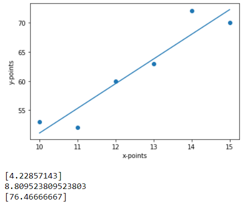
The above image is what your final output might look like. The 3 outputs below the plot are the response to our print() statements. So they are slope, intercept, and y_new respectively.
The equation of the regression line is y = 4.23x + 8.80. So according to the equation, when x = 16,
y= 4.23*(16) + 8.80 = 76.48. The small difference in the calculation is due to decimal points.
We can use .score() method that takes samples x and y as its 2 arguments to find R2 or the coefficient of determination. The best value for R2 is 1.0 and it can take negative values too, as the model can be worse. A closer value of R2 to 1.0 indicates the efficiency of our model.
linreg.score(xpoints, ypoints)
Run the code and you will see that the value of R2 is 0.89, so the model’s prediction is reliable.
What’s next?
This is as simple as a linear regression gets. It is not the only way but I found it to be the simplest and the easiest way. Don’t stop here. When you are comfortable with this, you can go one step ahead and consider a bigger dataset. For example, a CSV file. You will need to work with Pandas and NumPy packages in that case. Next, you can try a Multiple Linear or Logistic Regression Model. Keep learning and practicing.
The media shown in this article are not owned by Analytics Vidhya and is used at the Author’s discretion.


Thanks for this wonderful article about linear regression model.I got a small idea about it