Beginner’s Guide to Support Vector Machine(SVM)

Objective

• Learn how the support vector machine works
• Understand the role and types of kernel functions used in an SVM.

Introduction

Being a data science practitioner, you must be aware of the different algorithms available at our end. The important point is the awareness of when to use which algorithm. As an analogy, think of ‘Regression’ as a sword capable of slicing and dicing data efficiently, but incapable of dealing with highly complex data.

On the contrary, the ‘Support Vector Machine’ is like a sharp knife – it works on smaller datasets, but on complex ones, it can be much stronger and powerful in building machine learning models.

Note: If you are more interested in learning concepts in an Audio-Visual format, We have this entire article explained in the video below. If not, you may continue reading.

SVM is a supervised learning algorithm, that can be used for both classification as well as regression problems. However,  mostly it is used for classification problems. It is a highly efficient and preferred algorithm due to significant accuracy with less computation power.

In this article, we are going to see the working of SVM  and the different kernel functions used by the algorithm.

What is SVM?

In the SVM algorithm, we plot each observation as a point in an n-dimensional space (where n is the number of features in the dataset). Our task is to find an optimal hyperplane that successfully classifies the data points into their respective classes.

Before diving into the working of SVM let’s first understand the two basic terms used in the algorithm “The support vector ” and ” Hyper-Plane”.

Hyper-Plane

A hyperplane is a decision boundary that differentiates the two classes in SVM. A data point falling on either side of the hyperplane can be attributed to different classes. The dimension of the hyperplane depends on the number of input features in the dataset. If we have 2 input features the hyper-plane will be a line. likewise, if the number of features is 3, it will become a two-dimensional plane.

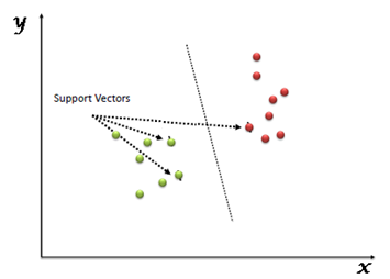
Support-Vectors

Support vectors are the data points that are nearest to the hyper-plane and affect the position and orientation of the hyper-plane. We have to select a hyperplane, for which the margin, i.e the distance between support vectors and hyper-plane is maximum. Even a little interference in the position of these support vectors can change the hyper-plane.

How SVM works?

As we have a clear idea of the terminologies related to SVM, let’s now see how the algorithm works. For example, we have a classification problem where we have to separate the red data points from the blue ones.

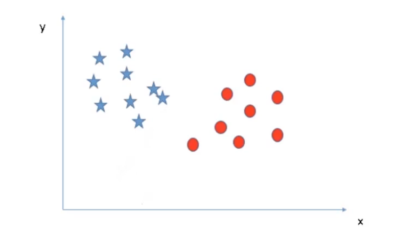
Since it is a two-dimensional problem, our decision boundary will be a line, for the 3-dimensional problem we have to use a plane, and similarly, the complexity of the solution will increase with the rising number of features.

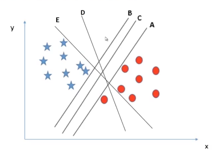
As shown in the above image, we have multiple lines separating the data points successfully. But our objective is to look for the best solution.

There are few rules that can help us to identify the best line.

Maximum classification, i.e the selected line must be able to successfully segregate all the data points into the respective classes. In our example, we can clearly see lines E and D are miss classifying a red data point. Hence, for this problem lines A, B, C is better than E and D. So we will drop them.

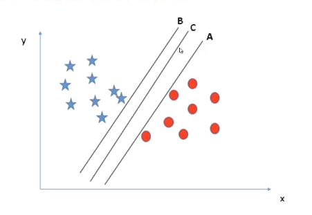
The second rule is Best Separation, which means, we must choose a line such that it is perfectly able to separate the points.

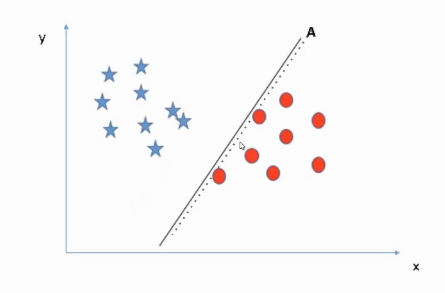
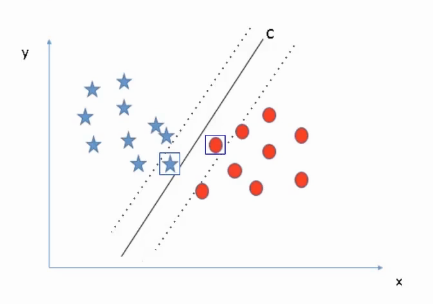
If we talk about our example, if we get a new red data point closer to line A as shown in the image below, line A will miss classifying that point. Similarly, if we got a new blue instance closer to line B, then line A and C will classify the data successfully, whereas line B will miss classifying this new point.

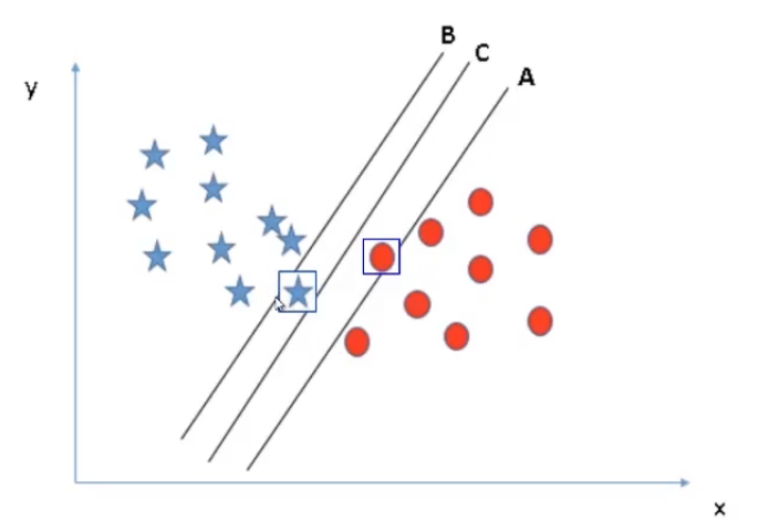
The point to be noticed here, In both the cases line C is successfully classifying all the data points why? To understand this let’s take all the lines one by one.

Why not Line A?

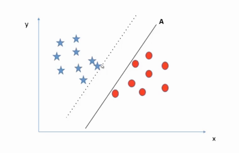
First, consider line A. If I move line A towards the left, we can see it has very little chance to miss classify the blue points. on the other hand, if I shift line A towards the right side it will very easily miss-classify the red points. The reason is on the left side of the margin i.e the distance between the nearest data point and the line is large whereas on the right side the margin is very low.

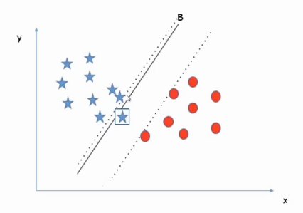
Why Not Line B?

Similarly, in the case of line B. If we shift line B towards the right side, it has a sufficient margin on the right side whereas it will wrongly classify the instances on the left side as the margin towards the left is very low. Hence, B is not our perfect solution.

Why Line C?

In the case of line C, It has sufficient margin on the left as well as the right side. This maximum margin makes line C more robust for the new data points that might appear in the future. Hence, C is the best fit in that case that successfully classifies all the data points with the maximum margin.

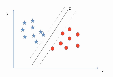
This is what SVM looks for, it aims for the maximum margin and creates a line that is equidistant from both sides, which is line C in our case. so we can say C represents the SVM classifier with the maximum margin.

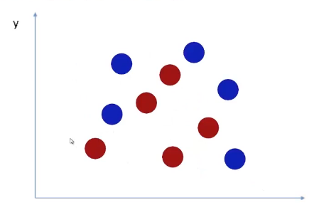
Now let’s look at the data below, As we can see this is not linearly separable data, so SVM will not work in this situation. If anyhow we try to classify this data with a line, the result will not be promising.

So, is there any way that SVM can classify this kind of data? For this problem, we have to create a decision boundary that looks something like this.

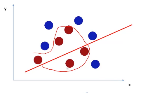
The question is, is it possible to create such a decision boundary using SVM. Well, the answer is Yes. SVM  does this by projecting the data in a higher dimension. As shown in the following image. In the first case, data is not linearly separable, hence, we project into a higher dimension.

If we have more complex data then SVM will continue to project the data in a higher dimension till it becomes linearly separable. Once the data become linearly separable, we can use SVM to classify just like the previous problems.

Projection into Higher Dimension

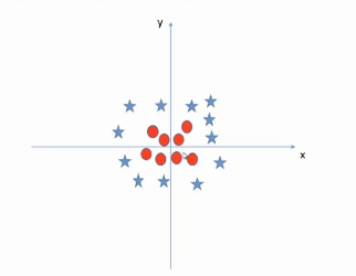
Now let’s understand how SVM projects the data into a higher dimension. Take this data, it is a circular non linearly separable dataset.

To project the data in a higher dimension, we are going to create another dimension z, where

Now we will plot this feature Z with respect to x, which will give us linearly separable data that looks like this.

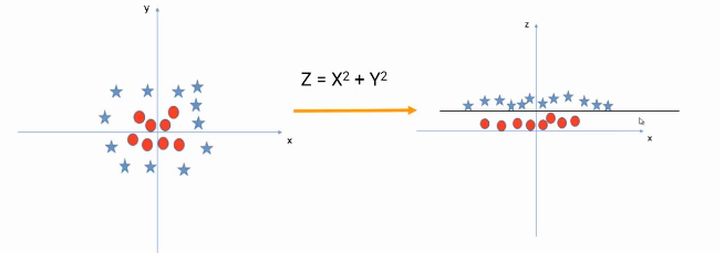
Here, we have created a mapping Z using the base features X and Y, this process is known as kernel transformation. Precisely, a kernel takes the features as input and creates the linearly separable data in a higher dimension.

Now the question is, do we have to perform this transformation manually? The answer is no. SVM handles this process itself, just we have to choose the kernel type.

Let’s quickly go through the different types of kernels available.

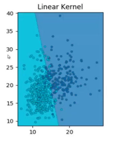
Linear Kernel

To start with, in the linear kernel, the decision boundary is a straight line. Unfortunately, most of the real-world data is not linearly separable, this is the reason the linear kernel is not widely used in SVM.

Gaussian / RBF kernel

It is the most commonly used kernel. It projects the data into a Gaussian distribution, where the red points become the peak of the Gaussian surface and the green data points become the base of the surface, making the data linearly separable.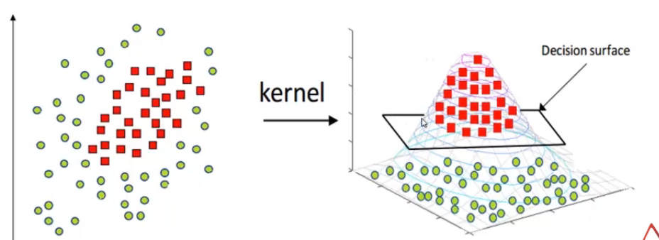

But this kernel is prone to overfitting and it captures the noise.

Polynomial kernel

At last, we have a polynomial kernel, which is non-uniform in nature due to the polynomial combination of the base features. It often gives good results.

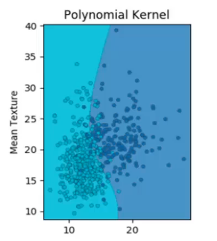
But the problem with the polynomial kernel is, the number of higher dimension features increases exponentially. As a result, this is computationally more expensive than RBF or linear kernel.

This is all about SVM in this article.

EndNote

To summarize in this article we tried to understand the working behind SVM, i.e how it chooses the optimal hyperplane to classify the data in respective classes. Also, we saw how the algorithm handles the complex data by projecting it into higher dimension space using kernel transformation.

If you are looking to kick start your Data Science Journey and want every topic under one roof, your search stops here. Check out Analytics Vidhya’s Certified AI & ML BlackBelt Plus Program

Let us know if you have any queries in the comments below.