Machine Learning with Python- Gaussian Naive Bayes

Introduction

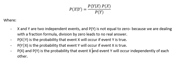
This article assumes that you possess a basic knowledge of Python, along with the basics of how a Machine Learning classifier functions. You will need to understand the basics concepts of the Pandas (Panel Data) and NumPy (Numerical Python) package. When we work with statistics and specifically probabilities, Gaussian Naive Bayes law is one of the most popular and fascinating theorems to dive into. The Bayesian theorem when working with statistics will allow you to calculate the probability that an event will occur provided that you have prior knowledge and information related to the specific event. Converted from text into a mathematical representation, the Gaussian Naive Bayes theorem appears as follows:

Source: My PC

Looking at the Naïve Bayes Law in Machine Learning context, one will find that the formula has differed slightly, however, the main idea of the formula is still retained. Because in Machine Learning there can exist multiple features, the Gaussian Naive Bayes formula has been mutated into the following:

Source: My PC

Training a Classifier with Python- Gaussian Naïve Bayes.

For this exercise, we make use of the “iris dataset”. This dataset is available for download on the UCI Machine Learning Repository.

We begin by importing the necessary packages as follows:

import pandas as pd
import numpy as np

We thereafter utilize the pandas “read_csv” method to load the data into our system. The pandas “read_csv” method will convert our data into a dataframe by default. A dataframe is simply a Python-generated spreadsheet-like object, i.e. it has rows and columns along with row indices and column names.

dataframe = pd.read_csv('iris_dataset.csv')

Before we take a look at the data, let us view some properties of our dataframe and indirectly, our data. We view the shape of the dataframe. The “shape” method will return to us a tuple of two integer values- the first value denotes the number of rows and the second, the number of columns.

print('The DataFrame Contains %d Rows And %d Columns'%(dataframe.shape))

We view the data type of the information that each feature contains. We make use of the “dtypes” method. From the below image, one can see that we have a dataframe that contains five features. Four out of five features contain floating-point values and one contains an object data type.

print(dataframe.dtypes)

Next, we shall check to see if any of our columns contain a null value. A “null” value is referring to a value or record that is missing. To do this, we make use of the “info” method. This method provides us with interesting information about our dataframe.

print(dataframe.info())

Now that we have gained a sufficient amount of insight into our data, let us view a portion of the dataframe. For this, pandas have a built-in method called “head”. By default, this method will return to us the first five rows of a dataframe. However, we can select the number of rows we wish to return by explicitly entering a value within the brackets.

print(dataframe.head(7))

As we can observe in the above image- we are now able to view raw values from the dataframe. For this problem we would like to predict the species that a flower may belong to, given values for the other features. Hence, it is time that we split the dataframe into the features matrix and target vector. With regards to this-, this requires that we manipulate the dataframe and it is for instances like these when the pandas’ indexers are very useful. Specifically the “loc” and “iloc” indexers.

features = dataframe.iloc[:, 0:4]

From the above image, we can observe that the features matrix has been created. It has been created by selecting all rows of the dataframe- a colon (:) denotes all- but from column zero (remember that python is zero-indexed, which means that the first element is assigned a value of 0 instead of 1) up until column four, and as we know python is exclusive of the end value. Hence, in reality, we selected all rows and columns zero up until three. Let us now print the first few rows of the features matrix.

print(features.head())

As expected, we observe that there are only four features/columns in the features matrix. Now, moving on to the target vector- it is time we isolate the values.

target = dataframe.iloc[:, -1]

Once again, we make use of the “iloc” indexer. This time, however, we select all rows of the dataframe, but only the last column. In Python’s lists, arrays, etc. you are allowed to index elements from the back of the list, array, etc. You can do this using negative index values- You will start from a negative one (-1) if you are indexing from the reverse direction. Hence we select all rows in the last column only as our target vector. Let us view the data stored in our target vector.

 print(target.head())

From the above image, we can confirm that we are on the right path up to this point in the problem. We have successfully loaded our data into the system, gained insight into our data, seen the nature and type of data we are working with, as well as configured our features matrix and target vector. Let us confirm the shapes of our initial dataframe, our new features matrix, and the target vector.

print('The Initial DataFrame Contained %d Rows And %d Columns'%(dataframe.shape))

print('The Features Matrix Contains %d Rows And %d Columns'%(features.shape))

print('The Target Vector Contains %d Rows And %d Columns'%(np.array(target).reshape(-1, 1).shape))

As expected,- Our dataframe contained an initial five columns, from which we decided we wanted to predict “species” hence giving us our target vector- which does contain one column and therefore leaving a remainder of four features which we see present in our features matrix. Now we shall instantiate a Gaussian Naïve Bayes, but first, we need to import the required package.

from sklearn.naive_bayes import GaussianNB
algorithm = GaussianNB(priors=None, var_smoothing=1e-9)

We have set the parameters and hyperparameters that we desire (the default values). Next, we proceed to conduct the training process. For this training process, we utilize the “fit” method and we pass in the data we wish to train the model on, i.e. the features matrix and target vector. During this process, the model learns how to utilize the values in the features matrix in the best possible way to reach the closest expected outcome.

algorithm.fit(features, target)

Once the training process is complete, you may view exactly how many different classes the model is trained to predict. We make use of the “classes_” method.

print(algorithm.classes_)

From the above output, we observe that our model has been trained to predict the species of iris that a flower may belong to. Three different species exist in our dataset and these are “Setosa”, “Versicolor”, “Virginia”. For information purposes, let us view the accuracy of our trained model. For this, we have the “score” method.

print('The Gaussian Model Has Achieved %.2f Percent Accuracy'%(algorithm.score(features, target)

Now, let us create a random observation to test whether or not the model functions effectively. We create an observation and use the “predict” method to predict future problems. The reason why we have four values in the two-dimensional array is that we have to pass in a value for each feature in the features matrix- Our feature matrix comprised four features- hence we pass a value for each feature. Based on the values we pass our model with the use of probability formulae to identify which species it will most likely belong to.

observation = [[5.0, 3.7, 1.6, 0.1]]

Now we shall print out the predicted species of plant.

print(predictions)

Our model has predicted this flower to belong to the “Setosa” species of iris flowers. Let us look at our model’s certainty.

print(algorithm.predict_proba(observation).round())

As we can observe three values are returned. Now, going back a bit, we remember that our classifier was trained to predict one of three species of iris flowers. Looking back we see that these species are (in the same order): Setosa, Versicolor, Virginia. And in the output of probabilities (above) we see the values 1, 0, 0. Now, the species and the probabilities are in their respective positions. This tells us that the model is 100% certain that the observation we created belongs to the “Setosa” species. It is %0 certain that it belongs to “Versicolor” or “Virginia”. Hence in our output, the model predicted “Setosa” as the species.

We have successfully trained and deployed a Machine Learning Classifier. This concludes my article on Gaussian Naive Bayes

Thank you for your time.

Shiv