The Architecture of Lenet-5

Objective

• Transfer learning through Pre-trained models is a time and cost-efficient solution for deep learning problems.
• Understand the Architecture of Lenet-5 as proposed by the authors.

Introduction

Suppose you want to learn a new subject. There are two ways to do that. One is to buy some books and start reading everything from scratch. The other way round is to go to a teacher and he will share all the knowledge and experience he has gained. Which process is faster and easier as well. Obviously, the second one i.e taking the help of a teacher.

Transfer learning works in a similar manner. Transfer learning is the method that uses a neural network trained on a large and generalized enough dataset and being used for another problem. These neural networks are called Pre-trained networks.

Note: If you are more interested in learning concepts in an Audio-Visual format, We have this entire article explained in the video below. If not, you may continue reading.

The basic requirement for transfer learning is the availability of a pre-trained network. Luckily, we have several state of the art deep learning networks shared by the respective teams. Like for computer vision we have

• Lenet-5
• Alexnet
• VGG16
• inception-v3
• Restnet

Out of these pre-trained networks, in this article, we are going to discuss Lenet-5 in detail.

What is Lenet5?

Lenet-5 is one of the earliest pre-trained models proposed by Yann LeCun and others in the year 1998, in the research paper Gradient-Based Learning Applied to Document Recognition. They used this architecture for recognizing the handwritten and machine-printed characters.

The main reason behind the popularity of this model was its simple and straightforward architecture. It is a multi-layer convolution neural network for image classification.

The Architecture of the Model

Let’s understand the architecture of Lenet-5. The network has 5 layers with learnable parameters and hence named Lenet-5. It has three sets of convolution layers with a combination of average pooling. After the convolution and average pooling layers, we have two fully connected layers. At last, a Softmax classifier which classifies the images into respective class.

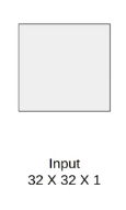
The input to this model is a 32 X 32 grayscale image hence the number of channels is one.

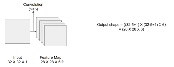
We then apply the first convolution operation with the filter size 5X5 and we have 6 such filters. As a result, we get a feature map of size 28X28X6. Here the number of channels is equal to the number of filters applied.

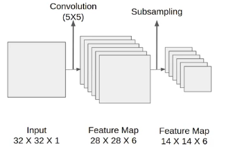
After the first pooling operation, we apply the average pooling and the size of the feature map is reduced by half. Note that, the number of channels is intact.

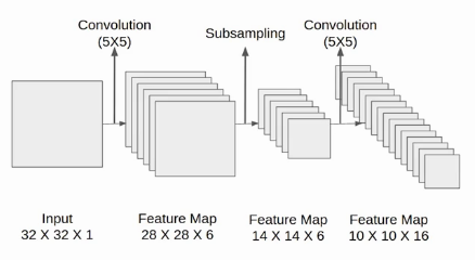
Next, we have a convolution layer with sixteen filters of size 5X5. Again the feature map changed it is 10X10X16. The output size is calculated in a similar manner. After this, we again applied an average pooling or subsampling layer, which again reduce the size of the feature map by half i.e 5X5X16.

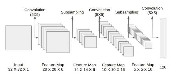
Then we have a final convolution layer of size 5X5 with 120 filters. As shown in the above image. Leaving the feature map size 1X1X120. After which flatten result is 120 values.

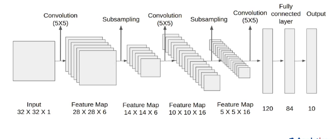
After these convolution layers, we have a fully connected layer with eighty-four neurons. At last, we have an output layer with ten neurons since the data have ten classes.

Here is the final architecture of the Lenet-5 model.

Architecture Details

Let’s understand the architecture in more detail.

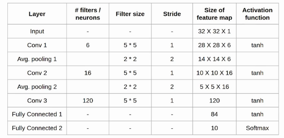
The first layer is the input layer with feature map size 32X32X1.

Then we have the first convolution layer with 6 filters of size 5X5 and stride is 1. The activation function used at his layer is tanh. The output feature map is  28X28X6.

Next, we have an average pooling layer with filter size 2X2 and stride 1. The resulting feature map is 14X14X6. Since the pooling layer doesn’t affect the number of channels.

After this comes the second convolution layer with 16 filters of 5X5 and stride 1. Also, the activation function is tanh. Now the output size is 10X10X16.

Again comes the other average pooling layer of 2X2 with stride 2. As a result, the size of the feature map reduced to 5X5X16.

The final pooling layer has 120 filters of 5X5  with stride 1 and activation function tanh. Now the output size is 120.

The next is a fully connected layer with 84 neurons that result in the output to 84 values and the activation function used here is again tanh.

The last layer is the output layer with 10 neurons and  Softmax function. The Softmax gives the probability that a data point belongs to a particular class. The highest value is then predicted.

This is the entire architecture of the Lenet-5 model. The number of trainable parameters of this architecture is around sixty thousand.

End Notes

This was all about Lenet-5 architecture. Finally, to summarize The network has

• 5 layers with learnable parameters.
• The input to the model is a grayscale image.
• It has 3 convolution layers, two average pooling layers, and two fully connected layers with a softmax classifier.
• The number of trainable parameters is 60000.

If you are looking to kick start your Data Science Journey and want every topic under one roof, your search stops here. Check out Analytics Vidhya’s Certified AI & ML BlackBelt Plus Program

If you have any queries, let me know in the comment section!