Hierarchical Modelling
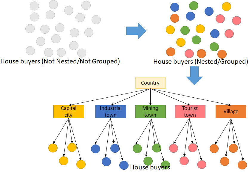
Hierarchical modeling also referred to as a nested model, deals with data with the observations in a certain group. There are some groups in hierarchical modeling with a number of observations and different groups can affect the target variable of the observation. In data analysis, we frequently find this kind of model. In this discussion, we will learn
- Hierarchical modeling; and
- Performing Mixed-effect regression.
Let’s start with a simple thing. Hierarchical modeling data frame consists of features and one target variable. Among the features, there is at least one numeric feature as the predictor. There is another categorical feature containing group information. For example, we want to study how personal annual income affects the purchased house price in 5 types of regions.
Annual income is the numeric predictor and the region type is the categorical feature to predict the house price. Higher-income affects higher purchased house prices. But, different type of region also affects how high the house price can be for the same annual income. The five types of regions we are discussing are the capital city, industrial town, mining town, tourist town, and village.
This is called hierarchical modeling because the observations are not mutually independent. The observations are grouped into 5 groups of region type and the region type also affects the house price. In other words, house price in the same region type is affected by unobserved variables, other than personal income.
To create a predictive model for this problem, we use mixed-effect regression assuming the annual income affects house price linearly. But, this is different from conventional linear regression as linear regression does not take into account the grouping, but treats all of the observations as mutually independent.
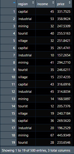
In this article, we will examine this simple fictive data. Below is how the data looks like. It has 500 observations with 100 observations for each region type. The annual income and house price units are in $’000. We will try to model mixed-effect linear regression equations for this data. Mixed-effect regression, like conventional linear regression, has an intercept and a slope. Intercept is the base value if the observed variable, in this case, is the income, is 0. The slope is the changing rate of the target variable (house price) for every increasing observed variable.
Conventional Linear Regression
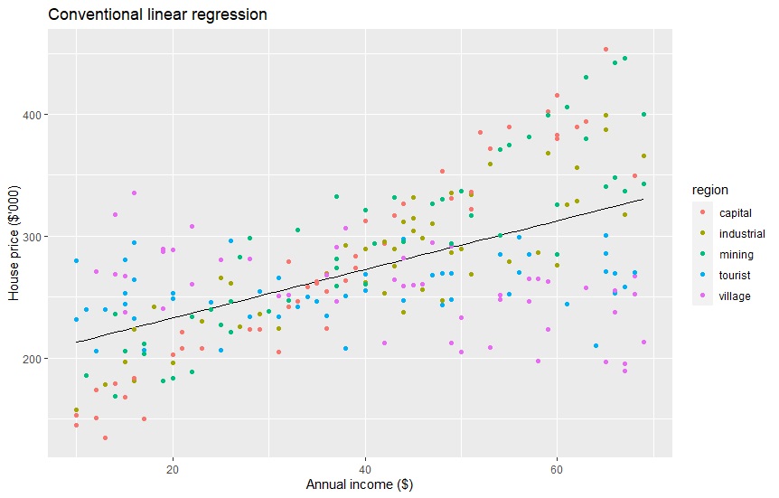
Before we perform the mixed-effect regression, we should try and see how conventional linear regression works. Conventional linear regression does not care about the region type. The equation form is y = a + bx, where y = house price, a = intercept, b = slope, and x = income. Below is the code and result on running the linear regression model, predicting using it, and visualize it. The equation from the code below is housePrice = 193 + 1.99*income. The RMSE is 48.95186. Later we will see mixed-effect regression having lower RMSE.
# Load packages
library(dplyr)
library(lme4)
library(ggplot2)
# 1. Conventional linear regression
conventional <- lm(price ~ income, data =  house_data)
summary(conventional)
#Call:
#lm(formula = price ~ income, data = house_data)
#
#Residuals:
#  Min      1Q  Median      3Q     Max
#-137.09  -30.25   -2.79   32.64  131.06
#
#Coefficients:
#  Estimate Std. Error t value Pr(>|t|)
#(Intercept) 193.0886     5.5270   34.94   <2e-16 ***
#  income        1.9929     0.1259   15.84   <2e-16 ***
#  ---
#  Signif. codes:  0 ‘***’ 0.001 ‘**’ 0.01 ‘*’ 0.05 ‘.’ 0.1 ‘ ’ 1
#
#Residual standard error: 49.05 on 498 degrees of freedom
#Multiple R-squared:  0.3349,     Adjusted R-squared:  0.3335
#F-statistic: 250.7 on 1 and 498 DF,  p-value: < 2.2e-16
# Extract coefficient
coef(conventional)
#(Intercept) distance
#193.088627 1.992909
confint(conventional)
#                 2.5 %     97.5 %
#(Intercept) 182.229607 203.947648
#income        1.745634   2.240183
# Predict
house_data$conventional <- predict(conventional)
# Visualize the data
ggplot(aes(x=income, y=conventional), data=house_data) +
  geom_line() +
  labs(x="Annual income ($)", y="House price ($'000)") +
  ggtitle("Conventional linear regression") +
  geom_point(data=house_data, aes(x=income, y=price, color=region))
# Evaluate the RMSE
rmse(house_data$price, house_data$conventional)
# 48.95186
Random-effect intercepts
We can see that the linear regression above cannot predict well because the residual errors are high. Many data points are far from the prediction. Mixed-effect regression can generate 5 linear equations for each of the region types. This assumes that each region type has unobserved information that can play a role in the prediction, so there should also be 5 equations.
In this article, we will try three kinds of mixed-effect regression. First, we will run random-effect intercepts with a fixed-effect slope. It means the 5 equations have different intercepts, but the same slope. The equation is expressed like this: y = ar + bx. The intercept a is different for each region.
# 2. Random effect: intercept
randomIntercept <- lmer(price ~ income  + (1|region), data=house_data)
summary(randomIntercept)
#Linear mixed model fit by REML ['lmerMod']
#Formula: price ~ income + (1 | region)
#Data: house_data
#
#REML criterion at convergence: 5270
#
#Scaled residuals:
#  Min      1Q  Median      3Q     Max
#-2.5103 -0.7306 -0.1011  0.6570  2.7977
#
#Random effects:
#  Groups   Name        Variance Std.Dev.
#region   (Intercept)  282.1   16.80
#Residual             2179.4   46.68
#Number of obs: 500, groups:  region, 5
#
#Fixed effects:
#  Estimate Std. Error t value
#(Intercept) 192.7179     9.1907   20.97
#income        2.0021     0.1207   16.58
#
#Correlation of Fixed Effects:
#  (Intr)
#income -0.530
# Extract coefficient
coef(randomIntercept)$region
#           (Intercept)   income
#capital       202.1464 2.002106
#industrial    195.5331 2.002106
#mining        212.6897 2.002106
#tourist       180.6501 2.002106
#village       172.5700 2.002106
# Predict
house_data$randomIntercept <- predict(randomIntercept)
# Visualize the data
ggplot(aes(x=income, y=randomIntercept, group=region, colour=region), data=house_data) +
  geom_line() +
  labs(x="Annual income ($)", y="House price ($'000)") +
  ggtitle("Random intercept") +
  scale_colour_discrete('Region')  +
  geom_point(data=house_data, aes(x=income, y=price, group=region, colour=region))
# Evaluate the RMSE
rmse(house_data$price, house_data$randomIntercept)
#46.41657
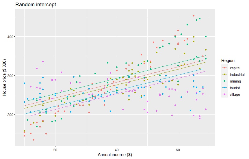
The five equations are below. The RMSE is 46.41657, a bit better than the previous one. But, the linear lines still do not fit the data points goods enough.
| Capital city | housePrice = 202 + 2.00*income |
| Industrial town | housePrice = 196 + 2.00*income |
| Mining town | housePrice = 213 + 2.00*income |
| Tourist town | housePrice = 181 + 2.00*income |
| Village | housePrice = 173 + 2.00*income |
Random-effect slopes
We can also apply random-effect to the slopes and fixed-effect to the intercept. The equation is expressed as y = a + brx. There will be 5 slopes based on region type with the same intercept.
# 3. Random Slope
randomSlope <- lmer(price ~ income  + (0 + income|region), data=house_data)
summary(randomSlope)
#Linear mixed model fit by REML ['lmerMod']
#Formula: price ~ income + (0 + income | region)
#Data: house_data
#
#REML criterion at convergence: 5118.2
#
#Scaled residuals:
#  Min      1Q  Median      3Q     Max
#-2.2973 -0.7671 -0.0084  0.6799  3.1690
#
#Random effects:
#  Groups   Name   Variance  Std.Dev.
#region   income    0.5234  0.7235
#Residual        1587.4197 39.8424
#Number of obs: 500, groups:  region, 5
#
#Fixed effects:
#  Estimate Std. Error t value
#(Intercept) 190.0637     4.5084  42.158
#income        2.0752     0.3395   6.112
#
#Correlation of Fixed Effects:
#  (Intr)
#income -0.279
# Extract coefficient
coef(randomSlope)$region
#           (Intercept)   income
#capital       190.0637 2.748727
#industrial    190.0637 2.228498
#mining        190.0637 2.734382
#tourist       190.0637 1.483813
#village       190.0637 1.180502
# Predict
house_data$randomSlope <- predict(randomSlope)
# Visualize the data
ggplot(aes(x=income, y=randomSlope, group=region, colour=region), data=house_data) +
  geom_line() +
  labs(x="Annual income ($)", y="House price ($'000)") +
  ggtitle("Random slope") +
  scale_colour_discrete('Region')  +
  geom_point(data=house_data, aes(x=income, y=price, group=region, colour=region))
# Evaluate the RMSE
rmse(house_data$price, house_data$randomSlope)
#39.6051
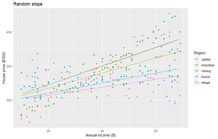
Here are the 5 equations. Applying random-effect slopes also has a bit lower RMSE, 39.6051.
| Capital city | housePrice = 190 + 2.75*income |
| Industrial town | housePrice = 190+ 2.23*income |
| Mining town | housePrice = 190 + 2.73*income |
| Tourist town | housePrice = 190 + 1.48*income |
| Village | housePrice = 190 + 1.18*income |
Random-effect intercepts and slopes
The last regression we are performing in this article is random-effect intercepts and slopes, with no fixed-effect, expressed as y = ar + brx. Now, each region type will have a different intercept and slope.
# 4. Random intercept and slope
randomBoth <- lmer(price ~ income + (1 + income|region), data=house_data)
summary(randomBoth)
#Linear mixed model fit by REML ['lmerMod']
#Formula: price ~ income + (1 + income | region)
#Data: house_data
#
#REML criterion at convergence: 4750.7
#
#Scaled residuals:
#  Min       1Q   Median       3Q      Max
#-2.87094 -0.56181  0.02465  0.67108  2.09393
#
#Random effects:
#  Groups   Name        Variance Std.Dev. Corr
#region   (Intercept) 3894.643 62.407
#income         3.453  1.858   -1.00
#Residual              743.616 27.269
#Number of obs: 500, groups:  region, 5
#
#Fixed effects:
#  Estimate Std. Error t value
#(Intercept) 187.4203    28.0830   6.674
#income        2.1721     0.8341   2.604
#
#Correlation of Fixed Effects:
#  (Intr)
#income -0.995
#optimizer (nloptwrap) convergence code: 0 (OK)
#Model failed to converge with max|grad| = 0.313943 (tol = 0.002, component 1)
# Extract coefficient
coef(randomBoth)$region
#           (Intercept)     income
#capital       95.18211  4.8908997
#industrial   159.31750  2.8874013
#mining       144.48934  3.6469465
#tourist      240.29470  0.4289196
#village      297.81792 -0.9935109
# Predict
house_data$randomBoth <- predict(randomBoth)
# Visualize the data
ggplot(aes(x=income, y=randomBoth, group=region, colour=region), data=house_data) +
  geom_line() +
  labs(x="Annual income ($)", y="House price ($'000)") +
  ggtitle("Random intercept and slope") +
  scale_colour_discrete('Region')  +
  geom_point(data=house_data, aes(x=income, y=price, group=region, colour=region))
# Evaluate the RMSE
rmse(house_data$price, house_data$randomBoth)
#26.94258
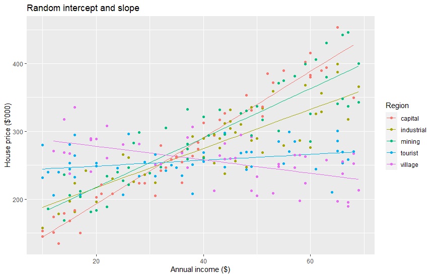
Random-effect slopes and intercepts result in 5 following equations. They have an RMSE of 26.94258, which is the lowest. Each line seems to nicely fit the data points by region type. We can examine that people in the capital city have the highest slope, but the lowest intercept.
It means that the increasing income of people in the capital city affects the most by increasing the house prices they purchased. Increasing income of people in the tourist town almost has no effect on the house price. We can also see a negative slope in the village group where people with higher income tend to spend less on their house prices.
| Capital city | housePrice = 95 + 4.89*income |
| Industrial town | housePrice = 159 + 2.89*income |
| Mining town | housePrice = 144 + 3.65*income |
| Tourist town | housePrice = 240 + 0.43*income |
| Village | housePrice = 298 + -0.99*income |
Next, I plan to write about paired tests as part two. The paired test is a hierarchical model where the same objects are observed repeatedly. We will see the difference between the times.
About author
Connect with me here https://www.linkedin.com/in/rendy-kurnia/
The media shown in this article are not owned by Analytics Vidhya and is used at the Author’s discretion.
A Data Science professional with seasoned specializations in Machine Learning development and Geo-spatial analysis. Hold the TensorFlow Developer Certificate. Have strong work experience in: - delivering meaningful data-driven insights to support business goals, - automating data processing, - data analysis (tabular, time series, text/NLP, and image), - descriptive and inferential statistical analysis, - GIS or spatial data analysis, - data visualization and dashboard development, - Machine Learning modeling (regression, classification, clustering, dimensionality reduction, time series forecasting, recommender engine) - Deep Learning or Artificial Intelligence (regression and classification with MLP, image classification with CNN, time series forecasting with LSTM, text classification with LSTM) - Hugging face: transformers, fine-tuning - Large Language Models (LLM) - Stable Diffusion - web application development, - developing APIs, etc.


This is really good knowledge sharing. Can you please write this for Python as well?
Excellent article! Clear and simple explanation. Thank you!