This article was published as a part of the Data Science Blogathon.
Introduction to GBM
One of the common ways to price a financial instrument is simulation. For stock price simulation, the simplest way is to assume the price follows Geometric Brownian Motion (GBM). With the simulated stock price, we can then price its derivative or other structure products.
The Geometric Brownian Motion (GBM) definition can be found in the Wiki.
In short, it assumes the rate of return of the stock price is under the Normal distribution and it can be expressed by the percentage drift μ and percentage volatility σ.
We express the rate of return as dS(t)/S(t), where dS(t) is the small delta change of the stock price S(t) between time t and t + dt
dS(t)/S(t) = μ * dt + σ * dW(t)
dW(t) is a random variable under normal distribution ~ N(0,t), which is called Wiener process.
The intuitive meaning of the above Stochastic Differential Equation (SDE) is that: the stock return will increase/decrease at the rate μ called drift, but mixed with the random noise under normal distribution with zero mean, and with the variance proportional to σ and time t. Thus, as time goes on, the uncertainty will increase.
Solving the SDE of the Geometric Brownian Motion(GBM), the stock price is under the Log-Normal distribution.
S(t) = S(0) exp( ( μ – σ^2 / 2 )t + σW(t) )
And its Expected Value and Variance are defined as:
E(S(t)) = S(0) exp(μt)
Var(S(t)) = S(0)^2 exp(2μt) ( exp(σ^2 * t) – 1 )
The key of the above formula is the input of the parameters: μ and σ. Traditionally, people use the sample mean and sample standard deviation as the approximation.
However, the parameters μ and σ may not necessarily be constant. From the Bayesian perspective, we can assume μ and σ under some probability distribution.
Bayesian Theory
I refer to my previous article — Introduction to probabilistic programming in Julia, for a recap on what is Bayesian Theory and Bayesian Inference.
In short, we can use the Julia package Turing.jl, which is designed for probabilistic programming, to estimate the probability distribution (aka. posterior probability distribution) of the parameters μ and σ by using the time-series dataset of stock price S(t).
The probabilistic model of the stock price is defined in the following Julia code segment, where “s” and “y” are the stock price time-series data. (“s” and “y” are the same data, we just use s1 as the initial price S(0), and y[i] is the price at the time “i” ).
@model GBM(s,y,n) = begin
    sig ~ Exponential(sample_std)
    u ~ Uniform(sample_mean - 2*sample_std,sample_mean + 2*sample_std)
    for i in 1:n
        if i == 1
            y[1] = s[1]
        else
            t = i-1
            mu = s[1]*exp(u * t)
            var = s[1]*s[1]*exp(2*u*t)*(exp(sig*sig*t)-1)
            y[i] ~ LogNormal(mu,sqrt(var))
        end
    end
end;
I found that the model convergency is quite sensitive to how we initialize the prior probability. As a reasonable initial value, we can initialize them with the sample mean (sample_mean) and the sample standard deviation (sample_std) of the stock price.
I iterated 1000 samplings on the GBM model (the code is shown below). In each invocation of the model GBM, we feed in time-series data as the arguments: i.e. the variable “train“, which stores the stock price data with size n. Then I repeated the 1000-iteration sampling by 5 times with the mapreduce function. The final result will be concatenated into the variable “chain”.
chain = mapreduce(c -> sample(GBM(train,train,n),NUTS(200, 0.65), 1000, discard_adapt=true),
    chainscat,
    1:5
)
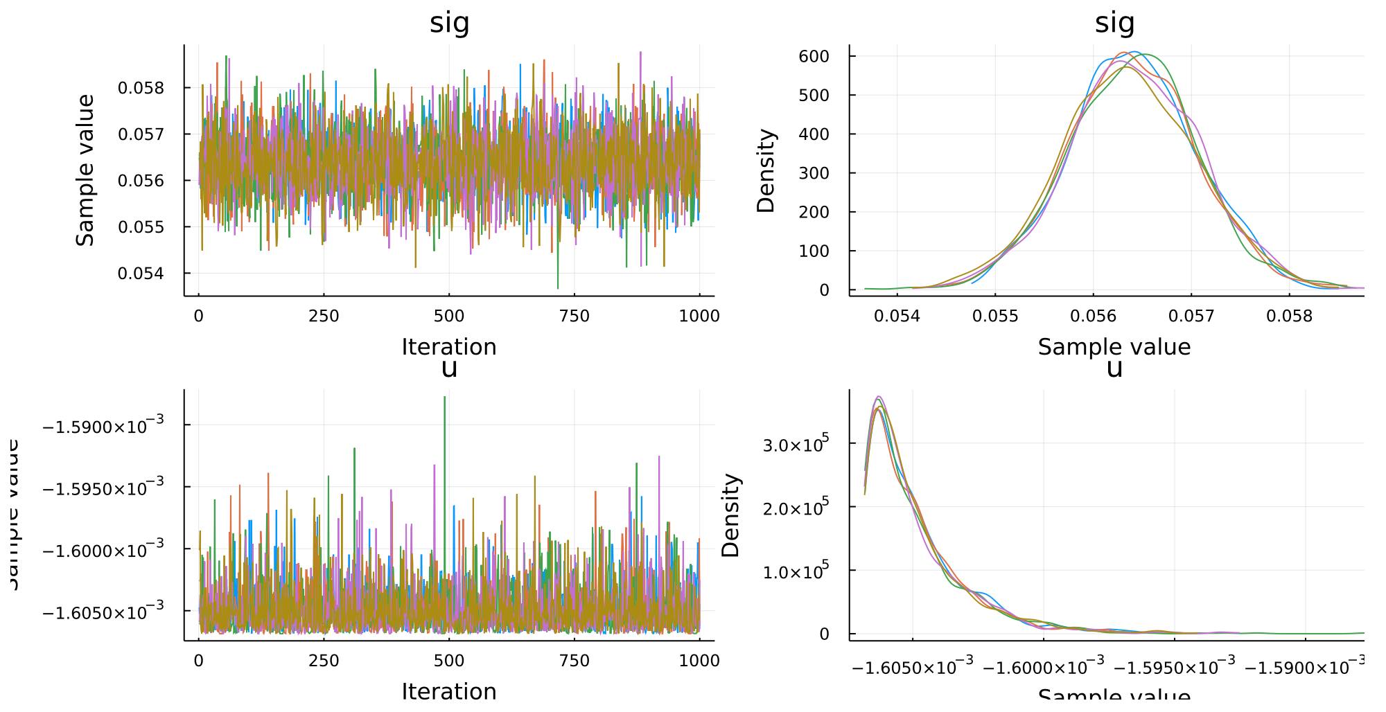
The graphs above showed the convergence of the simulation. The two graphs on the left column showed that the sample values of μ and σ are stable along with the 1000 iterations. The 5 lines in different colors represented the 5 chains of data. It is shown that they are overlapping closely, so we can say the results are stable.
The two graphs on the right column are the posterior distribution of μ and σ inferred by the simulation. The shapes of μ and σ are normal distribution and log-normal distribution respectively. Although μ and σ are initialized with Exponential distribution and Uniform distribution as the prior probability, at the end of the inference, the resulting posterior probability of μ and σ are normal distribution and log-normal distribution respectively. It is because, during the inference, the distribution of μ and σ will be corrected by the stock data (aka. evidence).
Stock Price Simulation
One of the advantages is that we can simulate the stock price using the posterior distribution instead of constant values. The chain contains 5000 pairs of μ and σ under the posterior distribution. Therefore we can sample μ and σ from the posterior probability distribution using the “chain” array.
The simulated stock price at time t is calculated by the following formula:
S(t) = S(t-dt) exp( ( μ – σ^2 / 2 )dt + σW(dt) )
The first component in the exponential: ( μ – σ^2 / 2 )*dt is the drift, and the second part: σW(dt) is the diffusion which contains the random part: W(dt) = epi[k,I] * sqrt(dt) where epi ~ Normal(0,1).
The stock prices along the time from 0 to T are simulated by N time steps. We divided the time T into N steps, so we have: dt = T/N. At each time step, the stock price at the previous time step is multiplied by the exponential of the sum of the drift and diffusion. We get the N random samples of μ and σ from chain[:u][:,] and chain[:sig][:,] which are supposed under the posterior probability distribution of μ and σ. As we use u[i] and sig[i] along with the time steps in the calculation of the drift and diffusion, the simulated stock prices along the time are calculated by varying μ and σ instead of constant μ and σ.
Here is the code to simulate the stock price with the posterior distribution of μ and σ.
function simulate_price(chain,s0,T,N)
    npath = 10
    y = zeros(Float32, npath, N)
    dt = convert(Float64,T) / convert(Float64,N)
    epi = rand(Normal(0,1),(npath,N))
    for k in 1:npath
       sig = sample(chain[:sig][:,], N)
        u = sample(chain[:u][:,] , N)
        for i in 1:N
            if i == 1
                y[k,1] = s0
            else
                drift = (u[i]-0.5*sig[i]*sig[i])*dt
                diffusion = sig[i]*epi[k,i]*sqrt(dt)
                y[k,i] = y[k,i-1]*exp(drift + diffusion)
            end
        end
    end
    return y
end;

paths = simulate_price(chain,train[1],5,50000)
Here we plot the graph of some of the simulated paths.
plot(paths[1,:])

plot!(paths[2,:])

plot!(paths[3,:])

plot!(paths[5,:])

plot!(paths[7,:])

plot!(paths[9,:])
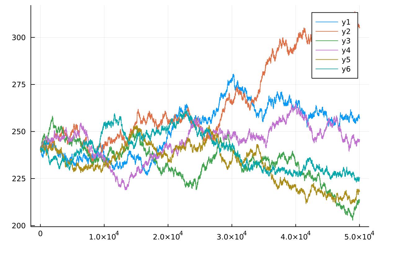
With these paths of stock price simulation, we can price the stock derivatives, e.g. the Call Option, by averaging the calculated payoff of the Call option based on the simulated stock price.
Let g(S'(T)) is the payoff function of the call option, S'(T) is the simulated stock price at the time T, then the price of the call option will be the present value of the average of the calculated payoff discounted by the risk-free rate (r):
C = E[ g(S'(T)) ] / (1+r)^T
Apart from the Call option, we can use the same way to price more complicated structured products as long as we can get the payoff function g(S'(T)) of the structured product.
The media shown in this article on Geometric Brownian Motion are not owned by Analytics Vidhya and is used at the Author’s discretion.


