This article was published as a part of the Data Science Blogathon
Introduction
This is Part-3 of the 4-part blog series on Bayesian Decision Theory.
In the previous article, we discussed the generalized cases for taking decisions in the Bayesian Decision Theory. Now, in this article, we will cover some new concepts including Discriminant Functions and Normal Density in Bayesian Decision Theory.
For previous articles, Links are Part-1 and Part-2.
The topics covered in this article are:
1. Classifiers, Discriminant Functions, and Decision Surfaces
2. The Normal Density
- Univariate normal density
- Multivariate normal density
Let’s get started,
Pattern classifiers can be represented in many different ways. Most used among all is using a set of discriminant function gi(x), i=1, . . . , c. The decision of the classifier works as assigning feature vector x to class wi– if a certain decision rule is to be followed like the followed earlier i.e.
gi(x) > gj(x) for j!=i
Hence this classifier can be viewed as a network that computes the c discriminant function and chooses the action to choose the state of nature that has the highest discriminant.

Fig. The functional structure of a general statistical pattern classifier includes d inputs and discriminant functions gi(x). A subsequent step determines which of the discriminant values is the maximum and categorizes the input pattern accordingly. The arrows show the direction of the flow of information, though frequently the arrows are omitted when the direction of flow is self-evident.
Image Source: Google Images
Generally gi(x) = -R(ai | x), for minimum conditional risk we get the maximum discriminant function.
Things can be further simplified by taking gi(x) = P(wi | x), so the maximum discriminant function corresponds to the maximum posterior probability.
Thus the choice of a discriminant function is not unique. We can temper the function by multiplying by the same positive constant or by shifting them by the same constant without any influence on the decision. These observations eventually lead to significant computational and analytical simplification. An example of discriminant function modification with tempering with the output decision is :
gi(x)= P(ωi|x)= p(x|ωi)P(ωi) / sum(p(x|ωj)P(ωj))
gi(x)= p(x|ωi)P(ωi)
gi(x)= ln p(x|ωi) + ln P(ωi)
There will be no change in the decision rule.
The aim of any decision rule is to divide the feature space into c decision regions, which are R1, R2, R3, . . , Rc. As discussed earlier if gi(x) >gj(x) for all j !=i, then x is in Ri, and the decision rule leads us to assign the features x to the state of nature wi. The regions are separated by decision boundaries.

Fig. In this two-dimensional two-category classifier, the probability densities are Gaussian, the decision boundary consists of two hyperbolas, and thus the decision region R2 is not simply connected. The ellipses mark where the density is 1/e times that at the peak of the distribution.
Image Source: Google Images
The Two Category Case
We can always build a dichotomizer (a special name for a classifier that classifies into two categories) for simplification. We used the decision rule that assigned x to w1 if g1 > g2, but we can define a single discriminant function,
g(x) ≡ g1(x) − g2(x),
And the decision rule decides w1 if g(x) > 0; otherwise it decides w2.
Hence dichotomizer can be seen as a system that computes a single discriminant function g(x) and classifies the x according to the sign of the output. The above equation can be further simplified as
g(x)= P(ω1|x) −P(ω2|x)
g(x)=ln(p(x|ω1)/ p(x|ω2)) + ln(P(w1)/P(w2))
Normal Density
Till now we are well aware that the Bayes classifiers are determined by class- conditional densities p(x|wi) and the priors. The most attractive density function that has been investigated is none other than multivariate normal density.
Further in this article, we get a brief exposition of multivariate normal density.
Univariate Normal density
The continuous univariate normal density p(x) can be given as,
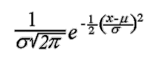
The expected value of x or the average or mean over the feature space.
𝜇 ≡ E [ x ] = Integration (from – ∞ to ∞ ): xp(x) dx
Variance is given as
σ2 ≡ E [ (x − μ)2 ] = Integration (from – ∞ to ∞ ): (x − μ)2p(x) dx
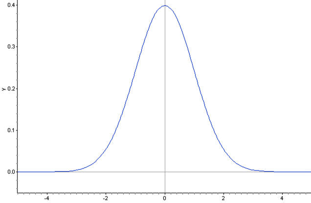
This density is fully governed by these two parameters: its mean and variance. We also write p(x)=N (𝜇, 𝜎2) which is read as x is distributed normally with the mean of 𝜇 and variance 𝜎2
The entropy of any distribution is given by
H(p(x)) = Integration (from – ∞ to ∞ ): p(x) ln p(x) dx
Which is measured in nats, but if log2 is used then the unit is a bit. The entropy of any distribution is a non-negative entity that given as an idea of fundamental uncertainty in the values of instances selected randomly from a distribution. As matter of fact, the normal distribution has the maximum entropy of all distribution having a given mean and variance.
Why Gaussian is Important?
The central limit theorem, states that the aggregated effect of a large number of small random independent disturbances will eventually lead to Gaussian distribution. Many real-life patterns -from handwritten characters to speech sounds — can be viewed as some ideal or prototype pattern corrupted by a large number of random processes.
Multivariate Normal Density
A multivariate normal distribution in dimensions of d is given as,
p(x) = (1/(2π)d/2|Σ|1/2 )exp[ −1/2(x − μ)tΣ−1(x − μ) ]
where,
x = d-component column vector
μ = d-component mean vector
Σ = d by d covariance matrix
|Σ| and Σ−1 are the determinant and inverse respectively
(x – μ)t is the transpose of (x – μ)
Some basic prerequisites are
Inner product
atb = sum(from i=1 to i=d): aibi
Mean
μ ≡ E [ x ] = Integration (from – ∞ to ∞ ): xp(x) dx
Covariance matrix
Σ ≡ E [(x − μ)(x − μ)t] = Integration (from – ∞ to ∞ ): (x − μ)(x − μ)tp(x) dx
If xi is the ith component of x, μi the ith component of μ, and σij the ijth component of Σ, then
μi = E [ xi ]
and,
σij = E [(xi − μi)(xj − μj)]
The covariance matrix holds a very important part of the discussion. The covariance matrix is always positive semidefinite and symmetric, here we will restrict our attention to the case in which the covariance matrix is positive definite, for the determinants to be positive.
σii are the variances and σij are the covariances. If σij =0 then xi and xj are statistically independent.
This ends today’s discussion!
In the next article, we will discuss the calculation of discriminant functions for normal density under different conditions and try to interpret all of those functions, and see the uses of all those cases in the real-life use-cases of Bayesian Decision Theory.
Discussion Problem
Determine the optimal decision boundary of Naive Bayes classifier where w = {w1, w2} and p(x|w1)= N(1, 1.5) and p(x|w2)= N(2, 2.5). Probability of prior is given as P(w1)= 1/7 and P(w2)=6/7 and loss matrix is given as [ [ 4, 3], [ 1, 2] ].
Note: Here N(x, y) indicates the normal density.
End Notes
Thanks for reading!
If you liked this and want to know more, go visit my other articles on Data Science and Machine Learning by clicking on the Link
Please feel free to contact me on Linkedin, Email.
Something not mentioned or want to share your thoughts? Feel free to comment below And I’ll get back to you.
About the author
Chirag Goyal
Currently, I am pursuing my Bachelor of Technology (B.Tech) in Computer Science and Engineering from the Indian Institute of Technology Jodhpur(IITJ). I am very enthusiastic about Machine learning, Deep Learning, and Artificial Intelligence.
The media shown in this article are not owned by Analytics Vidhya and is used at the Author’s discretion.
I am a B.Tech. student (Computer Science major) currently in the pre-final year of my undergrad. My interest lies in the field of Data Science and Machine Learning. I have been pursuing this interest and am eager to work more in these directions. I feel proud to share that I am one of the best students in my class who has a desire to learn many new things in my field.


