Complete Guide on Encoding Numerical Features in Machine Learning
Introduction
In Machine learning projects, we have features that could be in numerical and categorical formats. We know that Machine learning algorithms only understand numbers, they don’t understand strings. So, before feeding our data to Machine learning algorithms, we have to convert our categorical variables into numerical variables. However, sometimes we have to encode also the numerical features.
Why is there a need of encoding numerical features instead they are good for our Algorithms?
Let’s understand the answer to this question with an example,
Say we want to analyze the data of Google Play Store, where we have to analyze the Number of downloads of various applications. Since we know that all apps are not equally useful for users, only some popular applications are useful. So, there is a difference between the downloads for each one of those. Generally, this type of data is skewed in nature and we are not able to find any good insights from this type of data directly. Here is the need to encode our numerical columns to gain better insights into the data. Therefore, I convert numerical columns to categorical columns using different techniques. This article will discuss “Binning”, or “Discretization” to encode the numerical variables.
Techniques to Encode Numerical Columns
Discretization: It is the process of transforming continuous variables into categorical variables by creating a set of intervals, which are contiguous, that span over the range of the variable’s values. It is also known as “Binning”, where the bin is an analogous name for an interval.
Benefits of Discretization:
1. Handles the Outliers in a better way.
2. Improves the value spread.
3. Minimize the effects of small observation errors.
Types of Binning:
Unsupervised Binning:
(a) Equal width binning: It is also known as “Uniform Binning” since the width of all the intervals is the same. The algorithm divides the data into N intervals of equal size. The width of intervals is:
w=(max-min)/N
- Therefore, the interval boundaries are:
[min+w], [min+2w], [min+3w], – – – – – – – – – – – -, [min+(N-1)w] where, min and max are the minimum and maximum value from the data respectively. - This technique does not changes the spread of the data but does handle the outliers.
(b) Equal frequency binning: It is also known as “Quantile Binning”. The algorithm divides the data into N groups where each group contains approximately the same number of values.
- Consider, we want 10 bins, that is each interval contains 10% of the total observations.
- Here the width of the interval need not necessarily be equal.
Handles outliers better than the previous method and makes the value spread approximately uniform(each interval contains almost the same number of values).
(c) K-means binning: This technique uses the clustering algorithm namely ” K-Means Algorithm”.
- This technique is mostly used when our data is in the form of clusters.
Here’s the algorithm which is as followed:
Let X = {x1,x2,x3,……..,xn} be the set of observation and V = {v1,v2,…….,vc} be the set of centroids.
- Randomly select ‘c’ centroids(no. of centroids = no. of bins).
- Calculate the distance between each of the observations and centroids.
- Assign the observation to that centroid whose distance from the centroid is the minimum of all the centroids.
- Recalculate the new centroid using the mean(average) of all the points in the new cluster being formed.
- Recalculate the distance between each observation and newly obtained centroids.
- If no observation was reassigned in further steps then stop, otherwise, repeat from step (3) again.
Custom binning: It is also known as “Domain” based binning. In this technique, you have domain knowledge about your business problem statement and by using your knowledge you have to do your custom binning.
For Example, We have an attribute of age with the following values
Age: 10, 11, 13, 14, 17, 19, 30, 31, 32, 38, 40, 42, 70, 72, 73, 75
Now after Binning, our data becomes:
| Attribute | Age -1 | Age -2 | Age -3 |
| 10, 11, 13, 14, 17, 19 | 30, 31, 32, 38, 40, 42 | 70, 72, 73, 75 | |
| After Binning | Young | Mature | Old |
Implementation
This technique cannot be directly implemented using the Scikit-learn library like previous techniques, you have to use the Pandas library of Python and make your own logic to implement this technique.
Now, comes to the next technique which can also be used to encode numerical columns(features)
Binarization: It is a special case of Binning Technique. In this technique, we convert the continuous value into binary format i.e, in either 0 or 1.
For Example,
- Annual Income of the Population
If income is less than 5 lakhs, then that people include in the non-taxable region(Binary value -0), and if more than 5 lakhs, then includes in the taxable region(Binary value -1). - Very useful Technique in Image Processing, for converting a colored image into a black and white image.
As we know that image is the collection of pixels and its values are in the range of 0 to 255(colored images), then based on the selected threshold values you can binarize the variables and make the image into black and white, which means if less than that threshold makes that as 0 implies black portion, and if more than threshold makes as 1 means white portion.
Implementation: Uses binarizer class of Scikit-Learn library of Python, which has two parameters: threshold and copy. If we make the copy parameter True, then it creates a new column otherwise it changes in the initial column.
If you want to learn more about Binarizer class, then please refer to the Link
Implementation in Python
– To implement these techniques, we use the Scikit-learn library of Python.
– Class use from Scikit-learn : KBinsDiscretizer()
– You can find more about this class from this Link
Step-1: Import Necessary Dependencies
import pandas as pd
import numpy as np
Step-2: Import Necessary Packages
import matplotlib.pyplot as plt
from sklearn.model_selection import train_test_split
from sklearn.tree import DecisionTreeClassifier
from sklearn.metrics import accuracy_score
from sklearn.preprocessing import KBinsDiscretizer
from sklearn.compose import ColumnTransformer
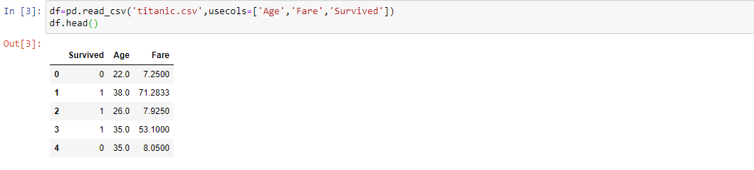
Step-3: Read and Load the Dataset
df=pd.read_csv('titanic.csv',usecols=['Age','Fare','Survived'])
print(df.head())
Step-4: Drop the rows where any missing value is present
df.dropna(inplace=True)
print(df.shape)
Step-5: Separate Dependent and Independent Variables
X=df.iloc[:,1:]
y=df.iloc[:,0]
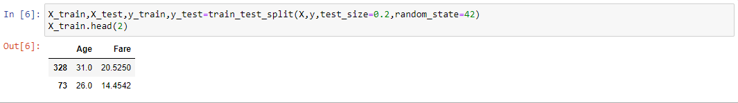
Step-6: Split our Dataset into Train and Test subsets
X_train,X_test,y_train,y_test=train_test_split(X,y,test_size=0.25,random_state=109)
print(X_train.head(2))
Step-7: Fit our Decision Tree Classifier
clf=DecisionTreeClassifier(criterion='gini')
clf.fit(X_train,y_train)
Step-8: Find the Accuracy of our model on the test Dataset
y_pred=clf.predict(X_test)
print(accuracy_score(y_test,y_pred))

Step-9: Form the objects of KBinsDiscretizer Class
Kbin_age=KBinsDiscretizer(n_bins=15,encode='ordinal',strategy='quantile')
Kbin_fare=KBinsDiscretizer(n_bins=15,encode='ordinal',strategy='quantile')
Step-10: Transform the columns using Column Transformer
trf=ColumnTransformer([('first',Kbin_age,[0]),('second',Kbin_fare,[1])])
X_train_trf=trf.fit_transform(X_train)
X_test_trf=trf.transform(X_test)
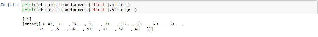
Step-11: Print the number of bins and the intervals point for the “Age” Column
print(trf.named_transformers_['first'].n_bins_)
print(trf.named_transformers_['first'].bin_edges_)
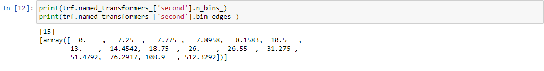
Step-12: Print the number of bins and the intervals point for the “Fare” Column
print(trf.named_transformers_['second'].n_bins_)
print(trf.named_transformers_['second'].bin_edges_)
Step-13: Fit-again our Decision Tree Classifier and check the accuracy
clf.fit(X_train_trf,y_train)
y_pred2=clf.predict(X_test_trf)
print(accuracy_score(y_test,y_pred2))
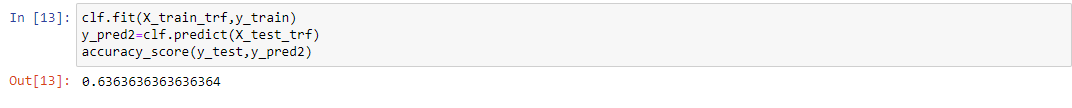
CONCLUSION: Here we observed that after applying the encoding techniques, there is an increment in the accuracy. Here, we only apply the Quantile Strategy, but you can try to change the “Strategy” parameter and then implement the different techniques accordingly.
End Notes
Thanks for reading!
If you liked this and want to know more, go visit my other articles on Data Science and Machine Learning by clicking on the Link
Please feel free to contact me on Linkedin, Email.
Something not mentioned or want to share your thoughts? Feel free to comment below And I’ll get back to you.
About the author
Chirag Goyal
Currently, I pursuing my Bachelor of Technology (B.Tech) in Computer Science and Engineering from the Indian Institute of Technology Jodhpur(IITJ). I am very enthusiastic about Machine learning, Deep Learning, and Artificial Intelligence.
The media shown in this article on How to encode numerical features are not owned by Analytics Vidhya and is used at the Author’s discretion.
I am currently pursuing my Bachelor of Technology (B.Tech) in Computer Science and Engineering from the Indian Institute of Technology Jodhpur(IITJ). I am very enthusiastic about Machine learning, Deep Learning, and Artificial Intelligence. Feel free to connect with me on Linkedin.


