Computer Vision Using OpenCV – With Practical Examples

This article was published as a part of the Data Science Blogathon

Introduction

OpenCV is a very famous library for computer vision and image processing tasks. It one of the most used pythons open-source library for computer vision and image data.

It is used in various tasks such as image denoising, image thresholding, edge detection, corner detection, contours, image pyramids, image segmentation, face detection and many more. If you want to know more about OpenCV, check this link.

📌 If you want to know about Python Libraries For Image Processing, then check this Link.

📌If you want to learn Image processing using NumPy, check this link.

📌 For more articles, click here

                                 Image Source

Table of Contents

• IMPORT LIBRARIES
• RGB IMAGE AND RESIZING
• GRAYSCALE IMAGE
• IMAGE DENOISING
• IMAGE THRESHOLDING
• IMAGE GRADIENTS
• EDGE DETECTION FOURIER TRANSFORM ON IMAGE
• LINE TRANSFORM
• CORNER DETECTION
• MORPHOLOGICAL TRANSFORMATION OF IMAGE
• GEOMETRIC TRANSFORMATION OF IMAGE
• CONTOURS
• IMAGE PYRAMIDS
• COLORSPACE CONVERSION AND OBJECT TRACKING
• INTERACTIVE FOREGROUND EXTRACTION
• IMAGE SEGMENTATION
• IMAGE INPAINTING
• TEMPLATE MATCHING
• FACE AND EYE DETECTION

IMPORT LIBRARIES 

Import all the required libraries using the below commands:

import os
import numpy as np
import cv2
import matplotlib.pyplot as plt
%matplotlib inline

RGB IMAGE AND RESIZING 

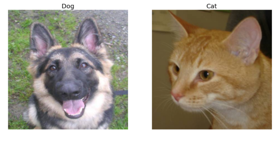
An RGB image where RGB indicates Red, Green, and Blue respectively can be considered as three images stacked on top of each other. It also has a nickname called ‘True Color Image’ as it represents a real-life image as close as possible and is based on human perception of colours.

The RGB colour model is used to display images on cameras, televisions, and computers.

Resizing all images to a particular height and width will ensure uniformity and thus makes processing them easier since images are naturally available in different sizes.

If the size is reduced, though the processing is faster, data might be lost in the image. If the size is increased, the image may appear fuzzy or pixelated. Additional information is usually filled in using interpolation.

height = 224
width = 224
font_size = 20
plt.figure(figsize=(15, 8))
for i, path in enumerate(paths):
name = os.path.split(path)[-1]
img = cv2.imread(path, cv2.IMREAD_COLOR)
resized_img = cv2.resize(img, (height, width))
plt.subplot(1, 2, i+1).set_title(name[ : -4], fontsize = font_size); plt.axis('off')
plt.imshow(cv2.cvtColor(resized_img, cv2.COLOR_BGR2RGB))
plt.show()

GRAYSCALE IMAGE 

Grayscale images are images that are shades of grey. It represents the degree of luminosity and carries the intensity information of pixels in the image. Black is the weakest intensity and white is the strongest intensity.

Grayscale images are efficient as they are simpler and faster than colour images during image processing.

plt.figure(figsize=(15, 8))
for i, path in enumerate(paths):
name = os.path.split(path)[-1]
img = cv2.imread(path, 0)
resized_img = cv2.resize(img, (height, width))
plt.subplot(1, 2, i + 1).set_title(f'Grayscale {name[ : -4]} Image', fontsize = font_size); plt.axis('off')
plt.imshow(resized_img, cmap='gray')
plt.show()

IMAGE DENOISING

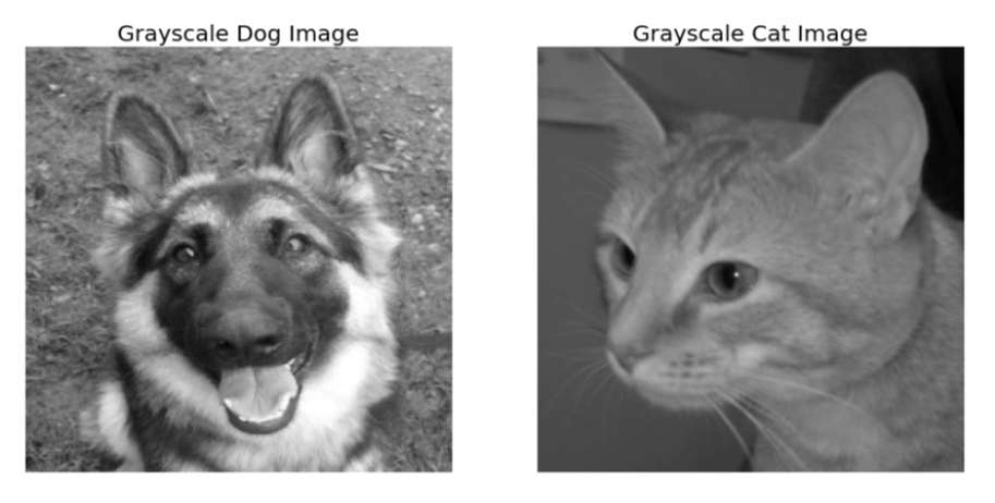
Image denoising removes noise from the image. It is also known as ‘Image Smoothing’. The image is convolved with a low pass filter kernel which gets rid of high-frequency content like edges of an image

for i, path in enumerate(paths):
name = os.path.split(path)[-1]
img = cv2.imread(path, cv2.IMREAD_COLOR)
resized_img = cv2.resize(img, (height, width))
denoised_img = cv2.medianBlur(resized_img, 5)
plt.figure(figsize=(15, 8))
plt.subplot(1, 2, 1).set_title(f'Original {name[ : -4]} Image', fontsize = font_size); plt.axis('off')
plt.imshow(cv2.cvtColor(resized_img, cv2.COLOR_BGR2RGB))
plt.subplot(1, 2, 2).set_title(f'After Median Filtering of {name[ : -4]} Image', fontsize = font_size); plt.axis('off')
plt.imshow(cv2.cvtColor(denoised_img, cv2.COLOR_BGR2RGB))
plt.show()

IMAGE THRESHOLDING

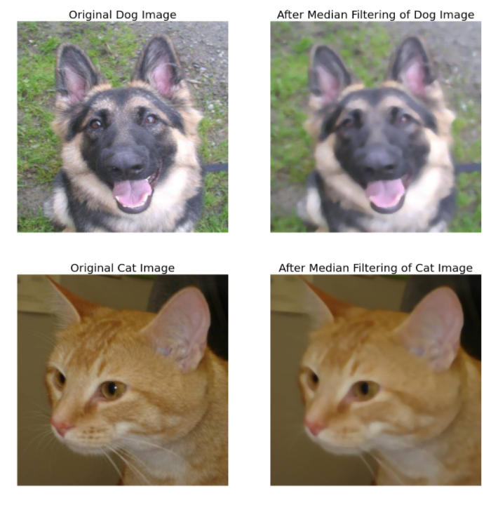
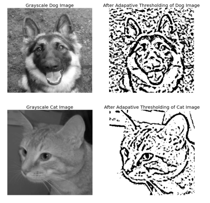
Image Thresholding is self-explanatory. If the pixel value in an image is above a certain threshold, a particular value is assigned and if it is below the threshold, another particular value is assigned.

Adaptive Thresholding does not have global threshold values. Instead, a threshold is set for a small region of the image. Hence, there are different thresholds for the entire image and they produce greater outcomes for dissimilar illumination. There are different Adaptive Thresholding methods

for i, path in enumerate(paths):
name = os.path.split(path)[-1]
img = cv2.imread(path, 0)
resized_img = cv2.resize(img, (height, width))
denoised_img = cv2.medianBlur(resized_img, 5)
th = cv2.adaptiveThreshold(denoised_img, maxValue = 255, adaptiveMethod = cv2.ADAPTIVE_THRESH_GAUSSIAN_C, thresholdType = cv2.THRESH_BINARY, blockSize = 11, C = 2)
plt.figure(figsize=(15, 8))
plt.subplot(1, 2, 1).set_title(f'Grayscale {name[ : -4]} Image', fontsize = font_size); plt.axis('off')
plt.imshow(resized_img, cmap = 'gray')
plt.subplot(1, 2, 2).set_title(f'After Adapative Thresholding of {name[ : -4]} Image', fontsize = font_size); plt.axis('off')
plt.imshow(cv2.cvtColor(th, cv2.COLOR_BGR2RGB))
plt.show()

IMAGE GRADIENTS

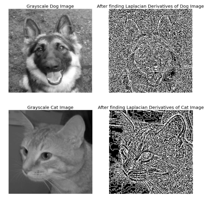
Gradients are the slope of the tangent of the graph of the function. Image gradients find the edges of a grayscale image in the x and y-direction. This can be done by calculating derivates in both directions using Sobel x and Sobel y operations.

for i, path in enumerate(paths):
name = os.path.split(path)[-1]
img = cv2.imread(path, 0)
resized_img = cv2.resize(img, (height, width))
laplacian = cv2.Laplacian(resized_img, cv2.CV_64F)
plt.figure(figsize=(15, 8))
plt.subplot(1, 2, 1).set_title(f'Grayscale {name[ : -4]} Image', fontsize = font_size); plt.axis('off')
plt.imshow(resized_img, cmap = 'gray')
plt.subplot(1, 2, 2).set_title(f'After finding Laplacian Derivatives of {name[ : -4]} Image', fontsize = font_size); plt.axis('off')
plt.imshow(cv2.cvtColor(laplacian.astype('float32'), cv2.COLOR_BGR2RGB))
plt.show()

EDGE DETECTION

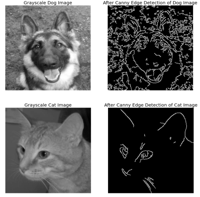
for i, path in enumerate(paths):
name = os.path.split(path)[-1]
img = cv2.imread(path, 0)
resized_img = cv2.resize(img, (height, width))
edges = cv2.Canny(resized_img, threshold1 = 100, threshold2 = 200)
plt.figure(figsize=(15, 8))
plt.subplot(1, 2, 1).set_title(f'Grayscale {name[ : -4]} Image', fontsize = font_size); plt.axis('off')
plt.imshow(resized_img, cmap = 'gray')
plt.subplot(1, 2, 2).set_title(f'After Canny Edge Detection of {name[ : -4]} Image', fontsize = font_size); plt.axis('off')
plt.imshow(cv2.cvtColor(edges, cv2.COLOR_BGR2RGB))

FOURIER TRANSFORM ON IMAGE 

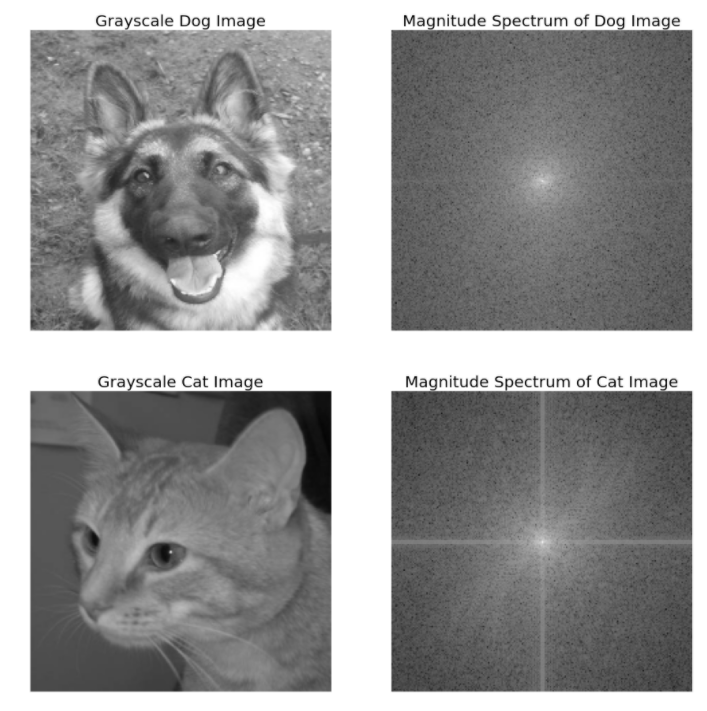
Fourier Transform analyzes the frequency characteristics of an image. Discrete Fourier Transform is used to find the frequency domain.

Fast Fourier Transform (FFT) calculates the Discrete Fourier Transform. Frequency is higher usually at the edges or wherever noise is present. When FFT is applied to the image, the high frequency is mostly in the corners of the image. To bring that to the centre of the image, it is shifted by N/2 in both horizontal and vertical directions.

Finally, the magnitude spectrum of the outcome is achieved. Fourier Transform is helpful in object detection as each object has a distinct magnitude spectrum

for i, path in enumerate(paths):
name = os.path.split(path)[-1]
img = cv2.imread(path, 0)
resized_img = cv2.resize(img, (height, width))
freq = np.fft.fft2(resized_img)
freq_shift = np.fft.fftshift(freq)
magnitude_spectrum = 20 * np.log(np.abs(freq_shift))
plt.figure(figsize=(15, 8))
plt.subplot(1, 2, 1).set_title(f'Grayscale {name[ : -4]} Image', fontsize = font_size); plt.axis('off')   
plt.imshow(cv2.cvtColor(resized_img, cv2.COLOR_BGR2RGB))
plt.subplot(1, 2, 2).set_title(f'Magnitude Spectrum of {name[ : -4]} Image', fontsize = font_size); plt.axis('off')   
plt.imshow(magnitude_spectrum, cmap = 'gray')
plt.show()

LINE TRANSFORM 

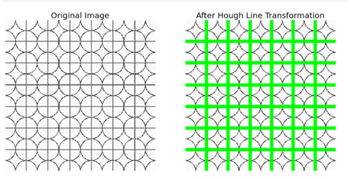
Hough Transform can detect any shape even if it is distorted when presented in mathematical form. A line in the cartesian coordinate system y = mx + c can be put in its polar coordinate system as rho = xcosθ + ysinθ. rho is the perpendicular distance from the origin to the line and θ is the angle formed by the horizontal axis and the perpendicular line in the clockwise direction.

So, the line is represented in these two terms (rho, θ). An array is created for these two terms where rho forms the rows and θ forms the columns. This is called the accumulator. rho is the distance resolution of the accumulator in pixels and θ is the angle resolution of the accumulator in radians.

For every line, its (x, y) values can be put into (rho, θ) values. For every (rho, θ) pair, the accumulator is incremented. This is repeated for every point on the line. A particular (rho, θ) cell is voted for the presence of a line.

This way the cell with the maximum votes implies a presence of a line at rho distance from the origin and at angle θ degrees.

min_line_length = 100
max_line_gap = 10
img = cv2.imread('../input/cv-images/hough-min.png')
resized_img = cv2.resize(img, (height, width))
img_copy = resized_img.copy()
edges = cv2.Canny(resized_img, threshold1 = 50, threshold2 = 150)
lines = cv2.HoughLinesP(edges, rho = 1, theta = np.pi / 180, threshold = 100, minLineLength = min_line_length, maxLineGap = max_line_gap)
for line in lines:
    for x1, y1, x2, y2 in line:
hough_lines_img = cv2.line(resized_img ,(x1,y1),(x2,y2),color = (0,255,0), thickness = 2)
plt.figure(figsize=(15, 8))
plt.subplot(1, 2, 1).set_title('Original Image', fontsize = font_size); plt.axis('off')   
plt.imshow(cv2.cvtColor(img_copy, cv2.COLOR_BGR2RGB))
plt.subplot(1, 2, 2).set_title('After Hough Line Transformation', fontsize = font_size); plt.axis('off')   
plt.imshow(cv2.cvtColor(hough_lines_img, cv2.COLOR_BGR2RGB))
plt.show()

CORNER DETECTION

img = cv2.imread('../input/cv-images/corners-min.jpg')
resized_img = cv2.resize(img, (height, width))
img_copy = resized_img.copy()
gray = cv2.cvtColor(resized_img,cv2.COLOR_BGR2GRAY)
gray = np.float32(gray)
corners = cv2.cornerHarris(gray, blockSize = 2, ksize = 3, k = 0.04)
corners = cv2.dilate(corners, None)
resized_img[corners > 0.0001 * corners.max()] = [0, 0, 255]
plt.figure(figsize=(15, 8))
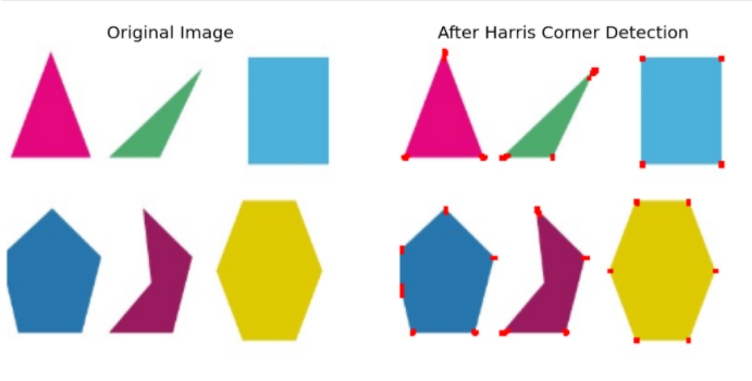
plt.subplot(1, 2, 1).set_title('Original Image', fontsize = font_size); plt.axis('off')   
plt.imshow(cv2.cvtColor(img_copy, cv2.COLOR_BGR2RGB))
plt.subplot(1, 2, 2).set_title('After Harris Corner Detection', fontsize = font_size); plt.axis('off')   
plt.imshow(cv2.cvtColor(resized_img, cv2.COLOR_BGR2RGB))
plt.show()

MORPHOLOGICAL TRANSFORMATION OF IMAGE 

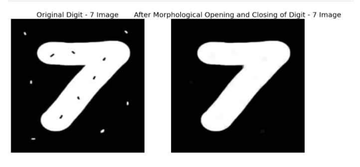
Morphological Transformation is usually applied on binary images where it takes an image and a kernel which is a structuring element as inputs. Binary images may contain imperfections like texture and noise.

These transformations help in correcting these imperfections by accounting for the form of the image

kernel = np.ones((5,5), np.uint8)
plt.figure(figsize=(15, 8))
img = cv2.imread('../input/cv-images/morph-min.jpg', cv2.IMREAD_COLOR)
resized_img = cv2.resize(img, (height, width))
morph_open = cv2.morphologyEx(resized_img, cv2.MORPH_OPEN, kernel)
morph_close = cv2.morphologyEx(morph_open, cv2.MORPH_CLOSE, kernel)
plt.subplot(1,2,1).set_title('Original Digit - 7 Image', fontsize = font_size); plt.axis('off')   
plt.imshow(cv2.cvtColor(resized_img, cv2.COLOR_BGR2RGB))
plt.subplot(1,2,2).set_title('After Morphological Opening and Closing of Digit - 7 Image', fontsize = font_size); plt.axis('off')   
plt.imshow(cv2.cvtColor(morph_close, cv2.COLOR_BGR2RGB))
plt.show()

GEOMETRIC TRANSFORMATION OF IMAGE 

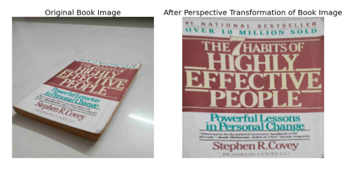
Geometric Transformation of images is achieved by two transformation functions namely cv2.warpAffine and cv2.warpPerspective that receive a 2×3 and 3×3 transformation matrix respectively.

pts1 = np.float32([[1550, 1170],[2850, 1370],[50, 2600],[1850, 3450]])
pts2 = np.float32([[0,0],[4160,0],[0,3120],[4160,3120]])
img = cv2.imread('../input/cv-images/book-min.jpg', cv2.IMREAD_COLOR)
transformation_matrix = cv2.getPerspectiveTransform(pts1, pts2)
final_img = cv2.warpPerspective(img, M = transformation_matrix, dsize = (4160, 3120))
img = cv2.cvtColor(img, cv2.COLOR_BGR2RGB)
img = cv2.resize(img, (256, 256))
final_img = cv2.cvtColor(final_img, cv2.COLOR_BGR2RGB)
final_img = cv2.resize(final_img, (256, 256))
plt.figure(figsize=(15, 8))    
plt.subplot(1,2,1).set_title('Original Book Image', fontsize = font_size); plt.axis('off')   
plt.imshow(img)
plt.subplot(1,2,2).set_title('After Perspective Transformation of Book Image', fontsize = font_size); plt.axis('off')   
plt.imshow(final_img)
plt.show()

CONTOURS 

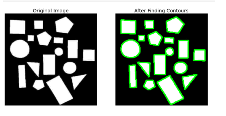
Contours are outlines representing the shape or form of objects in an image. They are useful in object detection and recognition. Binary images produce better contours. There are separate functions for finding and drawing contours.

plt.figure(figsize=(15, 8))
img = cv2.imread('contours-min.jpg', cv2.IMREAD_COLOR)
resized_img = cv2.resize(img, (height, width))
contours_img = resized_img.copy()
img_gray = cv2.cvtColor(resized_img,cv2.COLOR_BGR2GRAY)
ret,thresh = cv2.threshold(img_gray, thresh = 127, maxval = 255, type = cv2.THRESH_BINARY)
contours, hierarchy = cv2.findContours(thresh, mode = cv2.RETR_TREE, method = cv2.CHAIN_APPROX_NONE)
cv2.drawContours(contours_img, contours, contourIdx = -1, color = (0, 255, 0), thickness = 2)
plt.subplot(1,2,1).set_title('Original Image', fontsize = font_size); plt.axis('off')   
plt.imshow(resized_img)
plt.subplot(1,2,2).set_title('After Finding Contours', fontsize = font_size); plt.axis('off')   
plt.imshow(contours_img)
plt.show()

IMAGE PYRAMIDS 

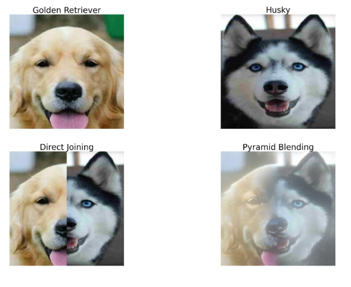
Images have a resolution which is the measure of the information in the image. In certain scenarios of image processing like Image Blending, working with images of different resolutions is necessary to make the blend look more realistic.

In OpenCV, images of high resolution can be converted to low resolution and vice-versa. By converting a higher-level image to a lower-level image, the lower-level image becomes 1/4th the area of the higher-level image.

When this is done for a number of iterations and the resultant images are placed next to each other in order, it looks like it is forming a pyramid and hence its name ‘Image Pyramid’

R = cv2.imread('GR-min.jpg', cv2.IMREAD_COLOR)
R = cv2.resize(R, (224, 224))
H = cv2.imread('../input/cv-images/H-min.jpg', cv2.IMREAD_COLOR)
H = cv2.resize(H, (224, 224))
G = R.copy()
guassian_pyramid_c = [G]
for i in range(6):
G = cv2.pyrDown(G)
guassian_pyramid_c.append(G)
G = H.copy()
guassian_pyramid_d = [G]
for i in range(6):
G = cv2.pyrDown(G)
guassian_pyramid_d.append(G)
laplacian_pyramid_c = [guassian_pyramid_c[5]]
for i in range(5, 0, -1):
GE = cv2.pyrUp(guassian_pyramid_c[i])
L = cv2.subtract(guassian_pyramid_c[i-1], GE)
laplacian_pyramid_c.append(L)
laplacian_pyramid_d = [guassian_pyramid_d[5]]
for i in range(5,0,-1):
guassian_expanded = cv2.pyrUp(guassian_pyramid_d[i])
L = cv2.subtract(guassian_pyramid_d[i-1], guassian_expanded)
laplacian_pyramid_d.append(L)
laplacian_joined = []
for lc,ld in zip(laplacian_pyramid_c, laplacian_pyramid_d):
r, c, d = lc.shape
lj = np.hstack((lc[:, 0 : int(c / 2)], ld[:, int(c / 2) :]))
laplacian_joined.append(lj)
laplacian_reconstructed = laplacian_joined[0]
for i in range(1,6):
laplacian_reconstructed = cv2.pyrUp(laplacian_reconstructed)
laplacian_reconstructed = cv2.add(laplacian_reconstructed, laplacian_joined[i])
direct = np.hstack((R[ : , : int(c / 2)], H[ : , int(c / 2) : ]))
plt.figure(figsize=(30, 20))
plt.subplot(2,2,1).set_title('Golden Retriever', fontsize = 35); plt.axis('off')   
plt.imshow(cv2.cvtColor(R, cv2.COLOR_BGR2RGB))
plt.subplot(2,2,2).set_title('Husky', fontsize = 35); plt.axis('off')   
plt.imshow(cv2.cvtColor(H, cv2.COLOR_BGR2RGB))
plt.subplot(2,2,3).set_title('Direct Joining', fontsize = 35); plt.axis('off')   
plt.imshow(cv2.cvtColor(direct, cv2.COLOR_BGR2RGB))
plt.subplot(2,2,4).set_title('Pyramid Blending', fontsize = 35); plt.axis('off')   
plt.imshow(cv2.cvtColor(laplacian_reconstructed, cv2.COLOR_BGR2RGB))
plt.show()

COLORSPACE CONVERSION AND OBJECT TRACKING 

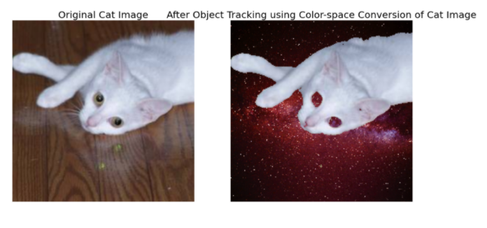
Colourspace Conversion, BGR↔Gray, BGR↔HSV conversions are possible. The BGR↔Gray conversion was previously seen. HSV stands for Hue, Saturation, and Value respectively.

Since HSV describes images in terms of their hue, saturation, and value instead of RGB where R, G, B are all co-related to colour luminance, object discrimination is much easier with HSV images than RGB images.

lower_white = np.array([0, 0, 150])
upper_white = np.array([255, 255, 255])
img = cv2.imread('../input/cv-images/color_space_cat.jpg', cv2.IMREAD_COLOR)
img = cv2.resize(img, (height, width))
background = cv2.imread("../input/cv-images/galaxy.jpg", cv2.IMREAD_COLOR)
background = cv2.resize(background, (height, width))
img = cv2.cvtColor(img, cv2.COLOR_BGR2RGB)
hsv_img = cv2.cvtColor(img, cv2.COLOR_BGR2HSV)
mask = cv2.inRange(hsv_img, lowerb = lower_white, upperb = upper_white)
final_img = cv2.bitwise_and(img, img, mask = mask)
final_img = np.where(final_img == 0, background, final_img)
plt.figure(figsize=(15, 8))
plt.subplot(1,2,1).set_title('Original Cat Image', fontsize = font_size); plt.axis('off')   
plt.imshow(img)
plt.subplot(1,2,2).set_title('After Object Tracking using Color-space Conversion of Cat Image', fontsize = font_size); plt.axis('off')   
plt.imshow(final_img)
plt.show()

INTERACTIVE FOREGROUND EXTRACTION 

The foreground of the image is extracted using user input and the Gaussian Mixture Model (GMM).

img = cv2.imread('Cat.jpg', cv2.IMREAD_COLOR)
img = cv2.resize(img, (height, width))
img_copy = img.copy()
mask = np.zeros(img.shape[ : 2], np.uint8)
background_model = np.zeros((1,65),np.float64)
foreground_model = np.zeros((1,65),np.float64)
rect = (10, 10, 224, 224)
cv2.grabCut(img, mask = mask, rect = rect, bgdModel = background_model, fgdModel = foreground_model, iterCount = 5, mode = cv2.GC_INIT_WITH_RECT)
new_mask = np.where((mask == 2) | (mask == 0), 0, 1).astype('uint8')
img = img * new_mask[:, :, np.newaxis]
plt.figure(figsize=(15, 8))
plt.subplot(1,2,1).set_title('Original Cat Image', fontsize = font_size); plt.axis('off')   
plt.imshow(cv2.cvtColor(img_copy, cv2.COLOR_BGR2RGB))
plt.subplot(1,2,2).set_title('After Interactive Foreground Extraction of Cat Image', fontsize = font_size); plt.axis('off')   
plt.imshow(cv2.cvtColor(img, cv2.COLOR_BGR2RGB))
plt.show()

IMAGE SEGMENTATION

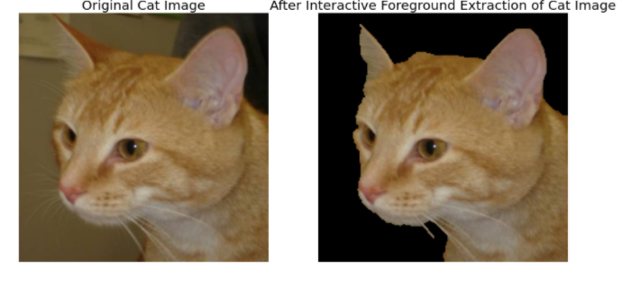
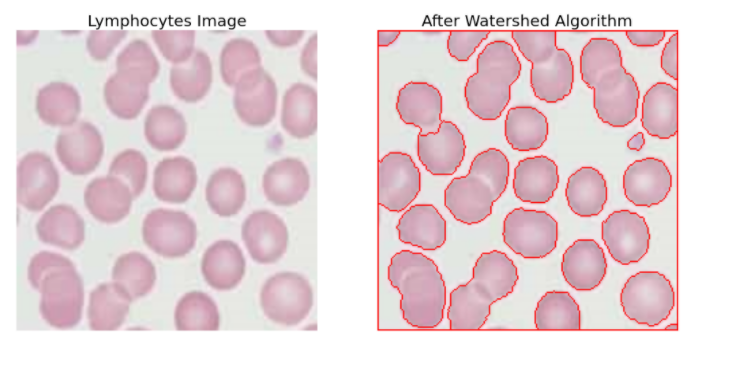
Image Segmentation is done using the Watershed Algorithm. This algorithm treats the grayscale image as hills and valleys representing high and low-intensity regions respectively. If these valleys are filled with coloured water and as the water rises, depending on the peaks, different valleys with different coloured water will start to merge.

To avoid this, barriers can be built which gives the segmentation result. This is the concept of the Watershed algorithm. This is an interactive algorithm as one can specify which pixels belong to an object or background. The pixels that one is unsure about can be marked as 0. Then the watershed algorithm is applied on this where it updates the labels given and all the boundaries are marked as -1

 img = cv2.imread('lymphocytes-min.jpg', cv2.IMREAD_COLOR)
resized_img = cv2.resize(img, (height, width))
img_copy = resized_img.copy()
gray = cv2.cvtColor(resized_img, cv2.COLOR_BGR2GRAY)
ret, thresh = cv2.threshold(gray, thresh = 0, maxval = 255, type = cv2.THRESH_BINARY_INV + cv2.THRESH_OTSU)
opening = cv2.morphologyEx(thresh, op = cv2.MORPH_OPEN, kernel = kernel, iterations = 2)
background = cv2.dilate(opening, kernel = kernel, iterations = 5)
dist_transform = cv2.distanceTransform(opening,cv2.DIST_L2,5)
ret, foreground = cv2.threshold(dist_transform, thresh = 0.2  * dist_transform.max(), maxval = 255, type = cv2.THRESH_BINARY)
foreground = np.uint8(foreground)
unknown = cv2.subtract(background, foreground)
ret, markers = cv2.connectedComponents(foreground)
markers = markers + 1
markers[unknown == 255] = 0
markers = cv2.watershed(resized_img, markers)
resized_img[markers == -1] = [0, 0, 255]
plt.figure(figsize=(15, 8))
plt.subplot(1, 2, 1).set_title('Lymphocytes Image', fontsize = font_size); plt.axis('off')   
plt.imshow(cv2.cvtColor(img_copy, cv2.COLOR_BGR2RGB))
plt.subplot(1, 2, 2).set_title('After Watershed Algorithm', fontsize = font_size); plt.axis('off')   
plt.imshow(cv2.cvtColor(resized_img, cv2.COLOR_BGR2RGB))
plt.show()

IMAGE INPAINTING 

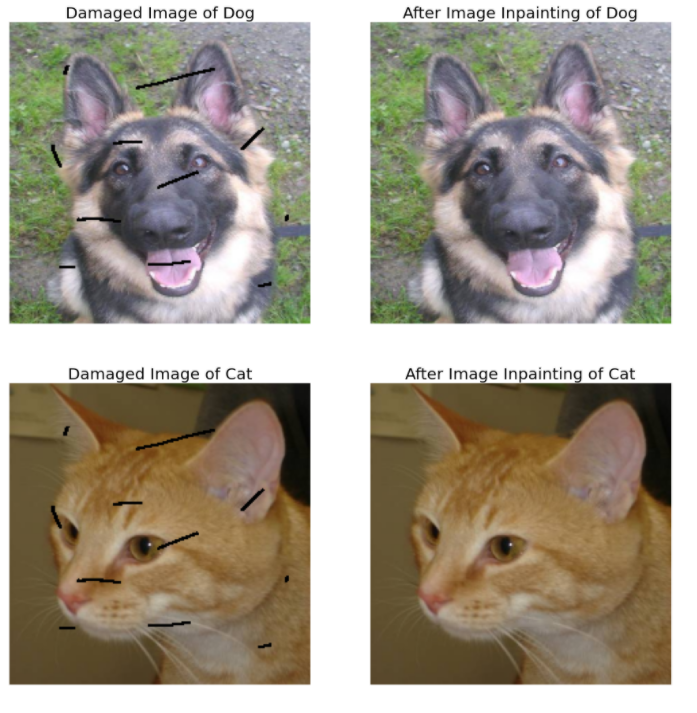
Images may be damaged and require fixing. For example, an image may have no pixel information in certain portions. Image Inpainting will fill all the missing information with the help of the surrounding pixels.

mask = cv2.imread('mask.png',0)
mask = cv2.resize(mask, (height, width))
for i, path in enumerate(paths):
name = os.path.split(path)[-1]
img = cv2.imread(path, cv2.IMREAD_COLOR)
resized_img = cv2.resize(img, (height, width))
ret, th = cv2.threshold(mask, 127, 255, cv2.THRESH_BINARY)
inverted_mask = cv2.bitwise_not(th)
damaged_img = cv2.bitwise_and(resized_img, resized_img, mask = inverted_mask)
result = cv2.inpaint(resized_img, mask, inpaintRadius = 3, flags = cv2.INPAINT_TELEA)
plt.figure(figsize=(15, 8))
plt.subplot(1, 2, 1).set_title(f'Damaged Image of {name[ : -4]}', fontsize = font_size); plt.axis('off')   
plt.imshow(cv2.cvtColor(damaged_img, cv2.COLOR_BGR2RGB))
plt.subplot(1, 2, 2).set_title(f'After Image Inpainting of {name[ : -4]}', fontsize = font_size); plt.axis('off')   
plt.imshow(cv2.cvtColor(result, cv2.COLOR_BGR2RGB))
plt.show()

TEMPLATE MATCHING 

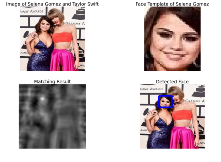
Template Matching matches the template provided to the image in which the template must be found. The template is compared to each patch of the input image. This is similar to a 2D convolution operation. It results in a grayscale image where each pixel denotes the similarity of the neighbourhood pixels to that of the template.

From this output, the maximum/minimum value is determined. This can be regarded as the top-left corner coordinates of the rectangle. By also considering the width and height of the template, the resultant rectangle is the region of the template in the image.

w, h, c = template.shape
method = eval('cv2.TM_CCOEFF')
result = cv2.matchTemplate(img, templ = template, method = method)
min_val, max_val, min_loc, max_loc = cv2.minMaxLoc(result)
top_left = max_loc
bottom_right = (top_left[0] + w, top_left[1] + h)
cv2.rectangle(img, top_left, bottom_right, color = (255, 0, 0), thickness = 3)
plt.figure(figsize=(30, 20))
plt.subplot(2, 2, 1).set_title('Image of Selena Gomez and Taylor Swift', fontsize = 35); plt.axis('off')
plt.imshow(cv2.cvtColor(img_copy, cv2.COLOR_BGR2RGB))
plt.subplot(2, 2, 2).set_title('Face Template of Selena Gomez', fontsize = 35); plt.axis('off')
plt.imshow(cv2.cvtColor(template, cv2.COLOR_BGR2RGB))
plt.subplot(2, 2, 3).set_title('Matching Result', fontsize = 35); plt.axis('off')
plt.imshow(result, cmap = 'gray')
plt.subplot(2, 2, 4).set_title('Detected Face', fontsize = 35); plt.axis('off')
plt.imshow(cv2.cvtColor(img, cv2.COLOR_BGR2RGB))
plt.show()

FACE AND EYE DETECTION

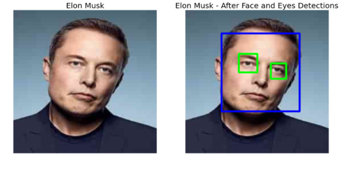
It is done by using Haar Cascades. Check the below code for face and eye detection:

face_cascade = cv2.CascadeClassifier(cv2.data.haarcascades + 'haarcascade_frontalface_default.xml')
eye_cascade = cv2.CascadeClassifier(cv2.data.haarcascades + 'haarcascade_eye.xml')
img = cv2.imread('../input/cv-images/elon-min.jpg')
img = cv2.resize(img, (height, width))
img_copy = img.copy()
gray = cv2.cvtColor(img, cv2.COLOR_BGR2GRAY)
faces = face_cascade.detectMultiScale(gray, scaleFactor = 1.3, minNeighbors = 5)
for (fx, fy, fw, fh) in faces:
img = cv2.rectangle(img, (fx, fy), (fx + fw, fy + fh), (255, 0, 0), 2)
roi_gray = gray[fy:fy+fh, fx:fx+fw]
roi_color = img[fy:fy+fh, fx:fx+fw]
eyes = eye_cascade.detectMultiScale(roi_gray)
    for (ex, ey, ew, eh) in eyes:
cv2.rectangle(roi_color, (ex, ey), (ex + ew, ey + eh), (0, 255, 0), 2)
plt.figure(figsize=(15, 8))
plt.subplot(1, 2, 1).set_title('Elon Musk', fontsize = font_size); plt.axis('off')   
plt.imshow(cv2.cvtColor(img_copy, cv2.COLOR_BGR2RGB))
plt.subplot(1, 2, 2).set_title('Elon Musk - After Face and Eyes Detections', fontsize = font_size); plt.axis('off')   
plt.imshow(cv2.cvtColor(img, cv2.COLOR_BGR2RGB))
plt.show()

End Notes

So in this article, we had a detailed discussion on Computer Vision Using OpenCV. Hope you learn something from this blog and it will help you in the future. Thanks for reading and your patience. Good luck!

You can check my articles here: Articles

Email id: [email protected]

Connect with me on LinkedIn: LinkedIn

The media shown in this article are not owned by Analytics Vidhya and is used at the Author’s discretion

Akshay Gupta 25 May 2021