Traditional vs Deep Learning Classification Models | An Empirical Study!

This article was published as a part of the Data Science Blogathon

1. Introduction

In this work, we present the relationship of model performance with varying dataset size and a varying number of target classes. We have performed our experiments on Amazon product reviews.

The dataset contains review title, review text and ratings. We have considered ratings as our output class. Further, We have performed three experiments (polarity 0/1), three class (positive, negative, neutral) and five class (1 to 5 rating). We have included three traditional and three deep learning models.

   Machine Learning Models 

1. Logistic Regression (LR)

2. Support Vector Machine (SVM)

3. Naive-Bayes (NB)

Deep Learning Models 

1. Convolution Neural Network (CNN)

2. Long Short Term Memory (LSTM)

3. Gated Recurrent Unit (GRU)

2.  The Dataset

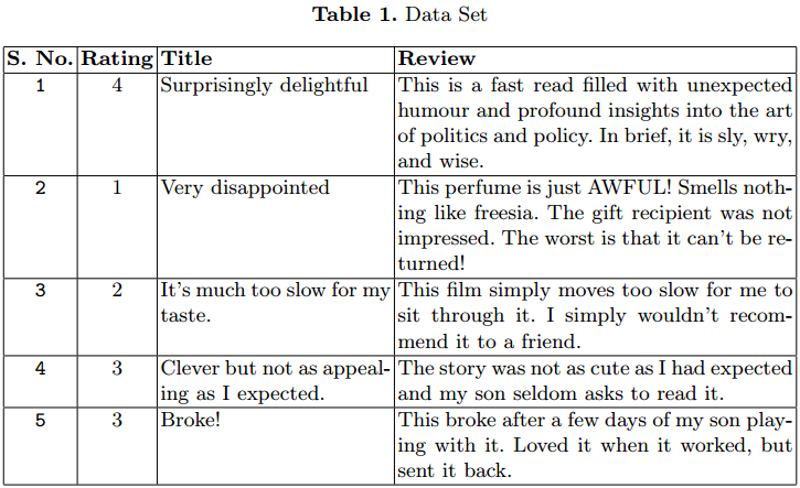
We use the amazon product review dataset for our experiment. The dataset contains 3.6 M instances of the product review in text form.

Separate train (3M) and test (0.6M) files have been provided in CSV format. Each instance has 3 attributes. The first attribute is the rating between 1 to 5. The second attribute is the title of the review. Last is the review text.

Some instances are given in Table 1. We have considered only 1.5 M.

3.  Experiment for Analysis

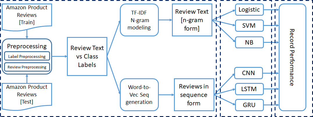
We have already mentioned that the whole experiment was performed for binary, three class, and five class classification. We have performed some preprocessing steps on the dataset before passing it to classification models. Each experiment was performed incrementally.

We started our training with 50000 instances and went up to 1.5 M instances for training. At last, we record the performance parameters for each model.

3.1 Preprocessing

 3.1.1 Label Mapping:

We have considered ratings as the class for the review text. The range of rating attribute is between 1 to 5. We need to map these ratings to the number of classes, considered for the particular experiment.

a) Binary Classification:-

Here, we map the rating 1 and 2 to class 0 and rating 4 and 5 to class 1. This form of classification can be treated as a sentiment classification problem, where the reviews with 1 and 2 ratings are in negative class, and 4 and 5 are in positive class.

We haven’t considered the reviews with a rating of 3 for the binary classification experiment. Hence we get fewer instances for the training comparing to the other two experiments.

b) Three Class Classification:-

Here, We extend our previous classification experiment. Now we consider rating 3 as a new separate class. New mapping of ratings to classes is as follows: Rating 1 and 2 mapped to class 0 (Negative), Rating 3 mapped to class 1 (Neutral) and rating 4 and 5 mapped to class 2 (Positive).

Instances for class 1 are very less than class 0 and 2, which creates a class imbalance problem. Therefore, we use micro-averaging while calculating performance measures.

c) Five Class Classification:-

Here, we consider each rating as a separate class. Mapping is as follows: Rating 1 mapped to class 0, Rating 2 mapped to class 1, Rating 3 mapped to class 2, Rating 4 mapped to class 3, and Rating 5 mapped to class 4.

3.1.2 Review Text Preprocessing:

Amazon product reviews are in text format. We need to convert the text data into a numerical format, which can be used for training the models.

For the Machine learning models, we convert the review text into TF-IDF vector format with the help of the sklearn library. Instead of taking each word individually, we consider the n-gram model while creating the TF IDF vectors. N-gram range is set to 2 – 3, and the max-feature value is set to 5000.

For Deep learning models, we need to convert text sequence data into numerical sequence data. We apply the word to vector modelling to convert each word into the equivalent vector.

The dataset contains a large number of words; hence, 1- hot encoding is very inefficient. Here we have used a pre-trained word2Vec model to represent each word with a column vector of size 300. We set the max length of the sequence equal to 70.

Reviews with word length less than 70 are padded with zeros at the starting. For the reviews with word length greater than 70, we select the first 70 words for word2Vec processing.

3.2 Classification model Training

We have mentioned earlier that we have taken three traditional machine learning models(LR, SVM, NB) and three deep learning models(CNN, LSTM, GRU). Preprocessed text with the label information is passed into models for training.

At first, We train all six models with 50000 instances and test them with 5000 instances. For the next iteration, we add 50000 and 5000 more instances in the train and test set respectively. We perform 30 iterations; hence, we consider 1.5 M, 150000 instances for train and test set in the last iteration.

The training mentioned above is performed for all three types of classifications experiments.

3.3 Model Configurations

We have used the default hyper-parameter settings of all the traditional classifiers used in this experiment. In CNN, the input size is 70 with an embedding size of 300. Embedding layer dropout is set to 0.3. 1-D convolution has been applied on the input, with the output size of convolution set to 100. Kernel size is kept to 3. Relu activation function has been used in the convolution layer. For the pooling process, Max-pooling is used. Adam’s Optimizer is used with a cross-entropy loss function.

LSTM and GRU also have the same hyper-parameter settings. The size of the output layer changes with the experiment under execution.

3.4 Performance Measures

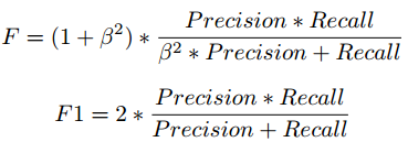
F score formula

We have taken the F1 score to analyze the performance of classification models with varying class labels and instance count. There is a trade-off between Precision and Recall if we try to improve Recall, Precision would be compromised, and the same applies in the reverse.

F1 score combines precision and recall in the form of harmonic mean.

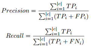
Precision, Recall formula in micro-averaging

In the three-class and five class classification, we observed that the count of instances with rating 3 is very less in the comparison of other ratings, which creates the class imbalance problem.

Hence we used the Micro-Averaging concept while calculating performance parameters. Micro-Averaging takes care of class imbalance while calculating the Precision and Recall. For detailed information on Precision, Recall please visit the following link: wiki link.

4 Results & Observation

In this section, we have presented the results of our experiments with varying dataset size and the number of class labels. A separate graph for each experiment has been presented. Graphs are plotted between the Test set size and the F1 score.

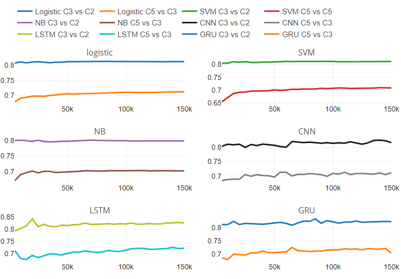
Additionally, we have provided Figure 5, which contains six subplots. Each subplot corresponds to one classifier. We have presented the rate of change between performance scores of two experiments concerning varying test set size.

Figure 2

Figure 2 presents the performance of classifiers on the binary classification task. Here actual test size is less than the data we have taken for testing because reviews with rating 3 have been removed.

Machine learning classifiers (LR, SVM, NB), perform constant except for slight variations at the starting points.

Deep Learning classifier (GRU and CNN) starts with less performance compared to SVM and LR. After three initial iterations, GRU and CNN continuously dominate the Machine learning classifiers.

The LSTM performs the most effective learning. LSTM started with the lowest performance. As the training set crosses 0.3 M, LSTM has shown continuous growth and ended with GRU.

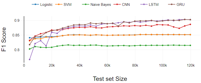
Fig 2. Binary classification performance analysis 

Figure 3

Figure 3, presents the three-class classification experiment results. The performance of all classifiers degrades as the classes increased. Performance is similar to binary classification if we compare a particular classifier with others.

The only difference is in the performance of LSTM. Here, LSTM has continuously increased performance unlike in the binary classification. LR performed a little better compared to SVM. Both LR and SVM performed equally in the Binary classification experiment.

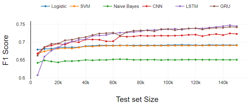
Fig 3. Three class classification performance analysis

Figure 4

Figure 4, represents the five-class classification experiment results. Results follow the same trends which appeared in the binary and three class classification experiment. Here the performance difference between LR and SVM increased a bit more.

Hence we can conclude that the LR and SVM performance gap increases as the number of classes increase.

From the overall analysis, Deep Learning classifiers perform better as the training dataset size increases and traditional classifiers show constant performance.

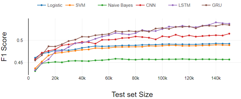
Fig 4. Five class classification performance analysis

Figure 5

Figure 5, represents the ratio of performance with respect to change in the number of classes and dataset size. The figure contains six subplots, one for each classifier. Each subplot has two lines; one line shows the performance ratio between three class and binary class classification on varying dataset size.

Another line is representing the performance ratio between five class and three class classification on varying dataset size. We have found that traditional classifiers have a constant rate of change. For traditional classifiers, the rate of change is independent of the dataset size. We can’t comment on the behaviour of Deep Learning models with respect to change in number classes and dataset size due to the variable pattern in the rate of change.

In addition to the experimental analysis mentioned above, we have analyzed the misclassified text data. We found interesting observations which affected the classification.

Sarcastic words:-

Customers wrote sarcastic product reviews. They have given the rating 1 or 2 but used so many positive polarity words. For example, one customer gave a rating of 1 and wrote the following review: “Oh! what a fantastic charger I got!!”. Classifier got confused with these type of polarity words and phrases.

Use of High Polarity words:-

Customers have given an average rating (3) but used highly polarized words in their reviews. For example, fantastic, tremendous, remarkable, pathetic, etc.

Use of Rare words:-

Having a dataset of size 3.6M, we still found so many uncommon words, which affected the classification performance. Misspelt, acronyms, short forms words used by reviewers are also important factors.

5. Endnote

We have analyzed the performance of traditional machine learning and deep learning models with varying dataset size and the number of the target class.

We have found that traditional classifiers can learn better than deep learning classifiers if the dataset is small. With the increase in the dataset size, deep learning models gain a boost in performance.

We have investigated the rate of change in classifier’s performance from binary to three class and three class to five class problem with varying dataset size.

We have used Keras deep learning library for experimentation. Results and Python scripts are available at the following link: GitHub Link.

The media shown in this article are not owned by Analytics Vidhya and is used at the Author’s discretion.