Feature Transformations in Data Science: A Detailed Walkthrough

Introduction

Data preprocessing is one of the many crucial steps of any Machine Learning project. As we know, our real-life data is often very unorganized and messy and without data preprocessing, there is no meaning in making a machine learning model. We have to first preprocess our data and then feed that processed data to our machine learning models for good performance. One part of preprocessing is Feature Transformation which we will discuss in this article.
Feature Transformation is a technique we should always use regardless of the model we are using, whether it is a classification task or regression task, or be it an unsupervised learning model.

What is Feature Transformation?

1. It is a technique by which we can boost our model performance. Feature transformation is a mathematical transformation in which we apply a mathematical formula to a particular column(feature) and transform the values which are useful for our further analysis.

2. It is also known as Feature Engineering, which is creating new features from existing features that may help in improving the model performance.

3. It refers to the family of algorithms that create new features using the existing features. These new features may not have the same interpretation as the original features, but they may have more explanatory power in a different space rather than in the original space.

4. This can also be used for Feature Reduction. It can be done in many ways, by linear combinations of original features or by using non-linear functions.

5. It helps machine learning algorithms to converge faster.

Why These Transformations?

1. Some Machine Learning models, like Linear and Logistic regression, assume that the variables follow a normal distribution. More likely, variables in real datasets will follow a skewed distribution.

2. By applying some transformations to these skewed variables, we can map this skewed distribution to a normal distribution so, this can increase the performance of our models.

Goal of Feature Transformations

As we know that Normal Distribution is a very important distribution in Statistics, which is key to many statisticians for solving problems in statistics. Usually, the data distribution in Nature follows a Normal distribution (examples like – age, income, height, weight, etc., ). But the features in the real-life data are not normally distributed, however it is the best approximation when we are not aware of the underlying distribution pattern.

Transformations present in scikit-learn

Sklearn has three Transformations-

1.  Function Transformation

2.  Power Transformation

3.  Quantile transformation

Function Transformations

LOG TRANSFORMATION:

– Generally, these transformations make our data close to a normal distribution but are not able to exactly abide by a normal distribution.

–  This transformation is not applied to those features which have negative values.

– This transformation is mostly applied to right-skewed data.

– Convert data from addictive Scale to multiplicative scale i,e, linearly distributed data.

RECIPROCAL TRANSFORMATION

– This transformation is not defined for zero.

– It is a powerful transformation with a radical effect.

– This transformation reverses the order among values of the same sign, so large values become smaller and vice-versa.

SQUARE TRANSFORMATION

–  This transformation mostly applies to left-skewed data.

SQUARE ROOT TRANSFORMATION:

– This transformation is defined only for positive numbers.

– This transformation is weaker than Log Transformation.

– This can be used for reducing the skewness of right-skewed data.

CUSTOM TRANSFORMATION

You can refer to the Link to read more about Function Transformations.

 Power Transformations

– Used when the desired output is more “Gaussian” like.

– Currently has ‘Box-Cox’ and ‘Yeo-Johnson’ transforms.

– Box-cox requires the input data to be strictly positive(not even zero is acceptable).

– for features that have zeroes or negative values, Yeo-Johnson comes to the rescue.

BOX-COX TRANSFORMATION:  Sqrt/sqr/log are the special cases of this transformation.

YEO-JOHNSON TRANSFORMATION:  It is a variation of the Box-Cox transform.

You can refer to the Link to read more about Power Transformations.

Implementation in Python

Function Transformations

Step-1: Import necessary Dependencies

import pandas as pd
import numpy as np
import scipy.stats as stats
import matplotlib.pyplot as plt
import seaborn as sns

Step-2: Import useful packages

from sklearn.model_selection import train_test_split
from sklearn.metrics import accuracy_score
from sklearn.model_selection import cross_val_score
from sklearn.linear_model import LogisticRegression
from sklearn.tree import DecisionTreeClassifier
from sklearn.preprocessing import FunctionTransformer

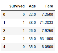
Step-3: Read and Load the dataset
Python Code:

import pandas as pd

df = pd.read_csv('titanic.csv',usecols=['Age','Fare','Survived'])
print(df.head())

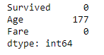
Step-4: Find the number of missing values per column

print(df.isnull().sum())

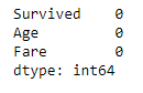
Step-5: Fill the missing values of the “Age” column with the median of the non-missing values

df['Age'].fillna(df['Age'].median(),inplace=True)

Step-6: Now, again check there is any missing value or not

print(df.isnull().sum())

Step-7: Separate independent and dependent variables

X = df.iloc[:,1:3]
y = df.iloc[:,0]

Step-8: Split our dataset into train and test subsets

X_train, X_test, y_train, y_test = train_test_split(X,y,test_size=0.33,random_state=105)

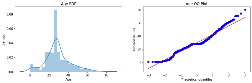
Step-9: Plot the probability density function(pdf) and the Q-Q plot for the “Age” column

import warnings
warnings.filterwarnings('ignore')
plt.figure(figsize=(10,2))
plt.subplot(121)
sns.distplot(X_train['Age'])
plt.title('Age PDF')
plt.subplot(122)
stats.probplot(X_train['Age'], dist="norm", plot=plt)
plt.title('Age QQ Plot')
plt.show()

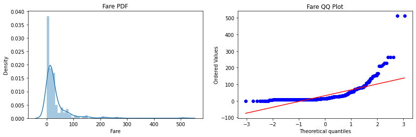
Step-10: Plot the probability density function(pdf) and the Q-Q plot for the “Fare” column

plt.figure(figsize=(10,2))
plt.subplot(121)
sns.distplot(X_train['Fare'])
plt.title('Age PDF')
plt.subplot(122)
stats.probplot(X_train['Fare'], dist="norm", plot=plt)
plt.title('Age QQ Plot')
plt.show()

Step-11: Form our Logistic Regression and Decision Tree Classifier

lr = LogisticRegression()
dt = DecisionTreeClassifier()

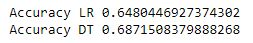
Step-12: Check the performance of both the classifiers on the test dataset(before transformation)

lr.fit(X_train,y_train)
dt.fit(X_train,y_train)
y_pred_lr = lr.predict(X_test)
y_pred_dt = dt.predict(X_test)
print("Accuracy LR",accuracy_score(y_test,y_pred_lr))
print("Accuracy DT",accuracy_score(y_test,y_pred_dt))

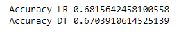
Step-13: Transform our dataset using log transformation and then repeat step-11 and step-12.

trf = FunctionTransformer(func=np.log1p)
X_train_transformed = trf.fit_transform(X_train)
X_test_transformed = trf.transform(X_test)
lr = LogisticRegression()
dt= DecisionTreeClassifier()
lr.fit(X_train_transformed,y_train)
dt.fit(X_train_transformed,y_train)
y_pred_lr = lr.predict(X_test_transformed)
y_pred_dt = dt.predict(X_test_transformed)
print("Accuracy LR",accuracy_score(y_test,y_pred_lr))
print("Accuracy DT",accuracy_score(y_test,y_pred_dt))

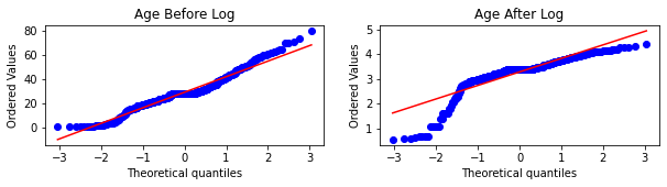
Step-14: Plot the probability density function(pdf) and the Q-Q plot for the “Age” column

plt.figure(figsize=(10,2))
plt.subplot(121)
stats.probplot(X_train['Age'], dist="norm", plot=plt)
plt.title('Age Before Log')
plt.subplot(122)
stats.probplot(X_train_transformed['Age'], dist="norm", plot=plt)
plt.title('Age After Log')
plt.show()

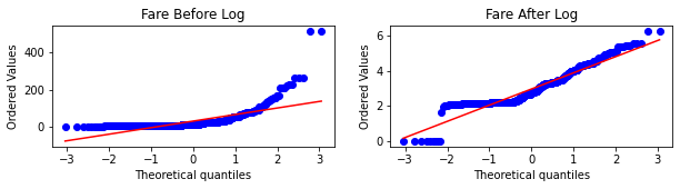
Step-15: Plot the probability density function(pdf) and the Q-Q plot for the “Fare” column

plt.figure(figsize=(10,2))
plt.subplot(121)
stats.probplot(X_train['Fare'], dist="norm", plot=plt)
plt.title('Fare Before Log')
plt.subplot(122)
stats.probplot(X_train_transformed['Fare'], dist="norm", plot=plt)
plt.title('Fare After Log')
plt.show()

Conclusion: Here, we implement the “Log-Transformation” but by changing the parameters inside the functions you can easily implement other transformations as well.

– The idea behind training two models is to verify that Tree-based model accuracy is not much affected by doing feature transformations, but models like Linear Regression, Logistic Regression performance increase up to some extent.

– How to Decide whether the given Q-Q plot corresponds to normal distribution or not?

In the Q-Q plots, if the variable follows a Normal distribution, then the variable’s values should fall in a line of slope 45-degree(y=x) when plotted against the theoretical quantiles.

– The main observation is that here the “Fare” column before transformation is right-skewed but after transformation comes closer to a normal distribution, but the “Age” column is not more affected since it is approx. normally distributed before the transformation.

– The accuracy of the model after doing transformation is increased for Logistic regression, but for verification of how much accuracy changes by transformation, you have to cross-validate over the data and find the average accuracy to gain better insights.

Power Transformations

Step-1: Import necessary Dependencies

import numpy as np
import pandas as pd
import seaborn as sns
import matplotlib.pyplot as plt
import scipy.stats as stats

Step-2: Import useful packages

from sklearn.model_selection import train_test_split
from sklearn.model_selection import cross_val_score
from sklearn.linear_model import LinearRegression
from sklearn.metrics import r2_score
from sklearn.preprocessing import PowerTransformer

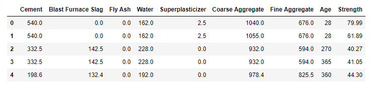
Step-3: Read and Load the dataset

df = pd.read_csv('concrete_data.csv')
df.head()

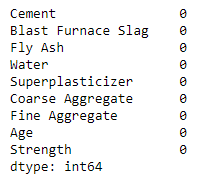
Step-4: Find the number of missing values per column

print(df.isnull().sum())

Step-5: Finding Statistical measures for columns

df.describe()

Step-6: Separate independent and dependent variables

X = df.iloc[:,:8]
y = df.iloc[:,-1]

Step-7: Split our dataset into train and test subsets

X_train, X_test, y_train, y_test = train_test_split(X,y,test_size=0.33,random_state=105)

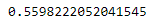
Step-8: Train our Linear Regression model and check the metric

lr = LinearRegression()
lr.fit(X_train,y_train)
y_pred = lr.predict(X_test)
print(r2_score(y_test,y_pred))

Step-9: Plotting the distplots without any transformation

import warnings
warnings.filterwarnings('ignore')
for col in X_train.columns:
    plt.figure(figsize=(14,4))
    plt.subplot(121)
    sns.distplot(X_train[col])
    plt.title(col)
    plt.subplot(122)
    stats.probplot(X_train[col], dist="norm", plot=plt)
    plt.title(col)
    plt.show()

Step-10: Apply the Box-Cox transformation

pt = PowerTransformer(method='box-cox')
X_train_transformed = pt.fit_transform(X_train+0.0000001)
X_test_transformed = pt.transform(X_test+0.0000001)
pd.DataFrame({'cols':X_train.columns,'box_cox_lambdas':pt.lambdas_})

Step-11: Train our model on transformed data and check the metric

lr = LinearRegression()
lr.fit(X_train_transformed,y_train)
y_pred2 = lr.predict(X_test_transformed)
print(r2_score(y_test,y_pred2))

Step-12: Plotting the distplots after transformation

X_train_transformed = pd.DataFrame(X_train_transformed,columns=X_train.columns)
for col in X_train_transformed.columns:
    plt.figure(figsize=(14,4))
    plt.subplot(121)
    sns.distplot(X_train[col])
    plt.title(col)
    plt.subplot(122)
    sns.distplot(X_train_transformed[col])
    plt.title(col)
    plt.show() 

Conclusion: Here we implement the Box-Cox transformation but by changing the parameters inside the function you can implement Yeo-Johnson Transformation also.

– The idea behind running the describe() function is to check the values present in the columns and verify the assumptions of Power Transformation i.e, Box-Cox transformation only accepts strictly positive numbers.

– We also observe that there is an increment in the accuracy of the model, since our problem statement is a “Regression” Problem statement and we apply the linear regression, and by transformations, we make the columns closer to a normal distribution, which satisfies the assumptions of the linear regression algorithm.

– We add a very small value to all the points of the dataset so that no point value remains exactly zero and our assumption still holds for Box-Cox transformation.

End Notes

Thanks for reading!

If you liked this and want to know more, go visit my other articles on Data Science and Machine Learning by clicking on the Link

Please feel free to contact me on Linkedin, Email.

Something not mentioned or want to share your thoughts? Feel free to comment below And I’ll get back to you.

Till then Stay Home, Stay Safe to prevent the spread of COVID-19, and Keep Learning!

About the Author

Chirag Goyal

Currently, I pursuing my Bachelor of Technology (B.Tech) in Computer Science and Engineering from the Indian Institute of Technology Jodhpur(IITJ). I am very enthusiastic about Machine learning, Deep Learning, and Artificial Intelligence.

Chirag Goyal

I am a B.Tech. student (Computer Science major) currently in the pre-final year of my undergrad. My interest lies in the field of Data Science and Machine Learning. I have been pursuing this interest and am eager to work more in these directions. I feel proud to share that I am one of the best students in my class who has a desire to learn many new things in my field.