Gradient Descent Algorithm : Understanding the Logic behind

This article was published as a part of the Data Science Blogathon

Introduction

Gradient Descent algorithm is an iterative algorithm used for the optimization of parameters used in an equation and to decrease the Loss (often called a Cost function). 

But before diving deep, we first need to have a basic idea of what a gradient means? Why are we calculating the gradient of a function and what is our final goal to achieve by using this algorithm?

The gradient of a function refers to the slope of the function at some point. We are calculating the gradient of a function to achieve the global minima of the function. And our goal is to achieve the best set of parameters (coefficients) for a function to have the minimum loss value.

Now, as we are aware of the to-do’s and the goal, let’s explore the concept gradually.

Y=b + w₁x₁+w₂x₂+w₃x₃ +…….+ w_mx_m  

Take an example of a simple linear equation of m-variables, representing a population sample. X₁, X₂, X₃…X_M (fig(a)).

Here in this equation, the number of parameters will be m+1 (X₁, X₂, X₃…X_M plus the intercept term).

Cost function

Now, writing the Cost function for the above linear equation.

Cost function (Loss) is calculated as an average of summation of square of (predicted values minus Actual values) as below:

 

As our objective was to find the global minima of the loss function, we need to plot the Loss function concerning all the parameters.

But we can see that the total number of dimensions for plotting the actual graph has become m+2. i.e. (m+1) parameters of actual equation plus the dependent variable i.e. loss. Plotting so many dimensions and interpreting is quite difficult. Hence, we need an iterative algorithm to reach the global minima of the function. The most common algorithm is the Gradient Descent algorithm.

Now we shall try to get the logic behind the scene of gradient descent.

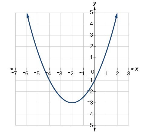
Let’s say this is our loss function

As seen above our loss function is a quadratic function. Suppose for our convenience this is our loss function, now if we want to calculate the gradient at x=1.5, we shall find it to be positive (1.66 approximately)  right? 

Now, the question is in which direction w.r.t x=1.5 we have to move to reach the minima. The trick is that we have to move opposite to the direction of the slope to reach the minima i.e. if the slope is positive then move in the negative direction and if the slope is negative then move in the positive direction. (Relate with the above diagram, as slope at x=1.5 ). Ok, now we get that, as the slope is positive at x=1.5 we have to move in the negative direction to search for the minima. But how much ??

So the second question that arises here is how much we have to move from point (1.5, 2.5) to get close to the minima of the function. This is called the learning rate. Suppose its “α”, so “α” determines the length of the stride by which we have to move in the negative direction. Learning rate should be chosen wisely as faster strides may lose the minima while extremely small learning rate will result in a long time to get to minima. So we should choose a learning rate between large and small values. Below is a simple diagram of the representation of strides to reach minima .

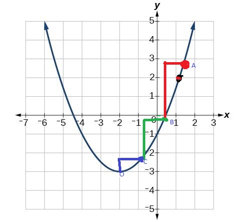
So, now as we are familiar with all the concepts needed for understanding this iterative algorithm, see the steps involved in this iterative process of the algorithm. For simplicity, we shall take a simple example of a linear equation of one variable and then generalize it for m terms: y=b+w₁x₁.

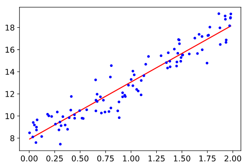
suppose the below figure represents a scatter plot of y vs variable x₁

 

OBJECTIVE:

To find the best set of parameters so as to minimize loss as much as possible (i.e. find the best value of w₁ and b to minimize the loss function), for more simplicity take intercept as zero.

In the above figure, we can figure out the loss for every data point as (predicted_value -actual_value)²

If we plot Loss vs parameter w₁ then we shall get a bowl-shaped graph like below.

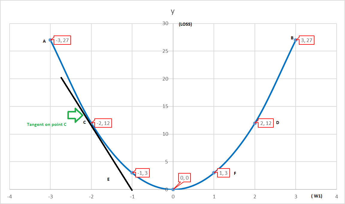
Here we can see that for each w₁ there would a loss associated with it. As here in our case, we are taking a simple model to understand, but we can imagine that as parameters increases, Dimensions increase (features). Hence, it will be very difficult for us to judge the minima visually.

Step_1: Initialize w₁ to any value (say point C in the above figure).

Step_2: Calculate the Loss function J(w₁, b).

Step_3: Take tangent to point C and calculate its gradient. We can find that the slope is negative for point C. So we shall move in the positive direction to reach minima.

Step_4: Deciding the Learning Rate ” α “

Step_5: w_1(new)= w_1(old) – α*(gradient)_w1

(Gradient shall decrease with each iteration and the length of stride will also get shorter)

Now, lets generalize the gradient descent algorithm for m+1 parameters.

y=b+w₁x₁+w₂x₂+w₃x₃+ ….. ….. +w_mx_m

(LOSS FUNCTION)   J(b,w)= 1/2  { Σ_{(i=1 to m)} [ h_w,b(x⁽ⁱ⁾ -y⁽ⁱ⁾]² } 

Step_1: First we shall randomly initialize b ,w₁,w₂,w₃…..w_m.

Step_2: Use all parameter values and predict h_w,b(x⁽ⁱ⁾) for each data point in the training data set.

Step_3: Calculate Loss J(b, w)

Step_4: Calculate Gradient of J(b ,w) w.r.t each parameters

Step_5: b_(new) = b _(old) – α (gradient)_b

w_1(new)=w_1(old) – α*(gradient)_w1

w_2(new)=w_2(old) – α*(gradient)_w2

Similarly for the m^th term    w _m(new)=w_m(old) – α*(gradient)_wm

Step_6: Update all parameters b , w₁ , w₂ ,w₃ , w₄ , .. w_m simultaneously.

Step_7: Go to Step_3.

Step_8: Repeat till convergence.

Now, we have a serious question that till when we should update our parameters and continue the iterative process. The answer is till the function converges. And how to check the Convergence let’s see :

Situation_1:

The graph of Loss vs parameters is purely convex: Then this is a simple case as we know a convex function converges when Slope ( Gradient ) is equal to zero.

So we shall be observing the parameter values either in subsequent iterations or for the past few iterations. If by observing the parameter values we get that the values are not significantly changing. In that case we can stop the training.

Situation_2:

If the Loss function is not purely convex or some tricky kind of function, like the graph below:

Here we can see that graph is going almost flat after some time. And we definitely don’t want to apply the algorithm forever.

So here the trick is to define the max number of steps. Defining the max number of steps is necessary as beyond a certain number of steps the parameter values don’t change significantly. So this is how we deal with the convergence part.

Handling the Gradient Descent Part of the calculation :

The gradient is nothing but a derivative of the loss function with respect to parameter values.

J(b,w)= 1/2 { Σ_{(i=1 to m)} [ h_w,bx⁽ⁱ⁾ -y⁽ⁱ⁾]² }     (parameters are w₁, w₂ … w_m and b ) 

Now calculate the partial derivative of the loss function with respect to parameter value (say w1)

 

 

 

Hence, in the same notion we can write general image source – self-sizing for any j^th parameter:

Also, we have to find the gradient concerning the constant term.

As we have the general representation of gradient with respect to all parameters including the constant. So, now we are in a position to write the most general form of representation, i.e.

The above equation is also called Batch Gradient Descent of “m” Data points as a batch of all m data points is trained together and post to that we update the parameters. When we complete one gradient descent update for all data points, it is called One Epoch.

As we have seen the calculation as well as the intuition of Gradient Descent and the concept of Batch Gradient Descent, we can now easily follow the concepts behind Mini-Batch Gradient Descent and Stochastic Gradient Descent.

Mini-Batch Gradient Descent :

Here we take a chunk of k-data points and calculate the Gradient Update. In each iteration, we are using exactly k-data points to calculate gradient descent update. If there are in total m data points and we are taking k-data points as a batch at a time then the number of batches per iterations can be calculated as ” m/k “.

(Usually, k is taken in the power of 2 like 32, 64,  512, 1024 )

Mini- Batch Gradient Descent works better than Gradient Descent as parameters get updated with every gradient update of the batch of data.

Now, we shall see a special case of Gradient Descent in which batch size k=1. This is called Stochastic gradient descent.

Stochastic Gradient Descent (sgd) :(k=1) Here we update the gradient just by looking at a single data point. Just after training on one data point, the gradient is updated. 

Steps for mini-batch gradient descent and stochastic gradient descent.

Step_1: Draw a bunch of k-examples of data points. (X⁽ⁱ⁾ ,Y⁽ⁱ⁾)

Step_2: Randomly Initialize parameters.

Step_3: Repeat until convergence.

Step_4: Obtain predictions from the model and calculate Loss on the Batch. (In stochastic process Batch size is of only one data point.)

Step_5: Calculate the gradient of the loss with respect to each parameter.

Step_6: Update the parameters simultaneously.

Conclusion

Finally, we have attained our objective of learning gradient descent and understanding the logic behind batch and stochastic gradient descent.

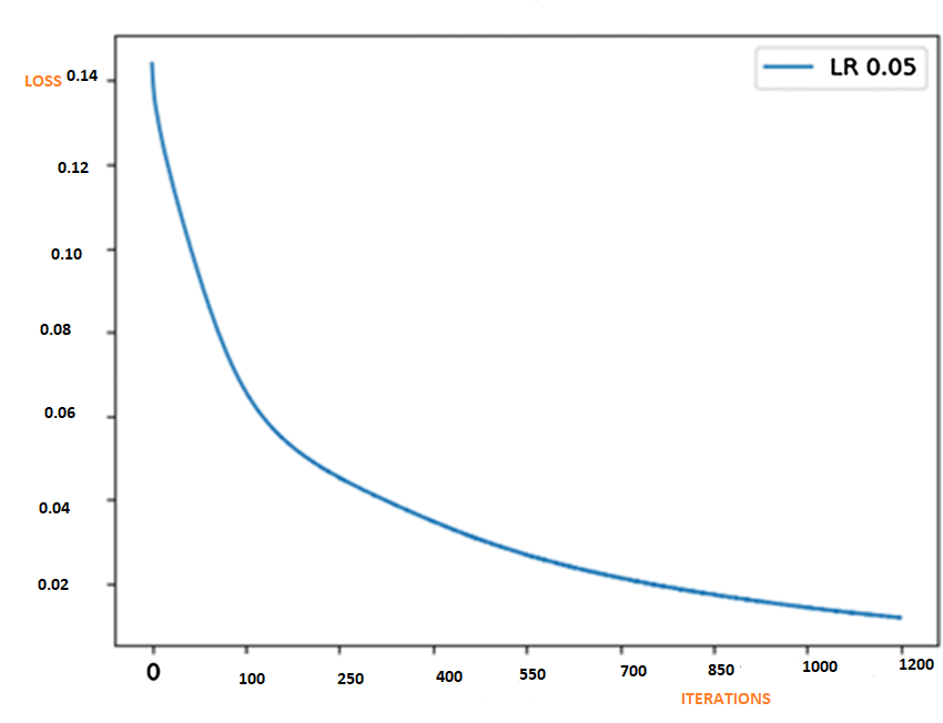
But as these all are optimization algorithms i.e. used for fetching the best set of parameters, you might be having the question that how do we know that our model is learning??

Well, in that case, we can plot the graph of Loss vs Iteration. The logic says loss should reduce with an increasing number of iterations just like the graph below. (Note LR is the learning rate we have seen i.e. ” α ” ).

The media shown in this article are not owned by Analytics Vidhya and are used at the Author’s discretion.