Introduction
Decision trees are versatile tools in machine learning, providing interpretable models for classification and regression tasks. Enhancing their performance, Chi-Square Automatic Interaction Detection (CHAID) offers a method for feature selection.
This article explores the implementation of the CHAID algorithm in decision trees. We’ll first learn about decision trees and the chi-quare test, followed by the practical implementation of CHAID using Python’s scikit-learn library. With step-by-step guidance and code examples, we’ll learn how to integrate CHAID into machine learning workflows for improved accuracy and interoperability.

Learning Objectives
- Understand the rationale behind using decision trees as one of the best supervised learning methods.
- Learn about the chi-square statistic and its role in the CHAID algorithm.
- Implement a decision tree using the CHAID algorithm in Python for classification tasks.
- Gain insights into interpreting CHAID decision tree results by analyzing the split decisions based on categorical variables.
This article was published as a part of the Data Science Blogathon!
Table of Contents
What are Decision Trees?
Decision tree learning or classification Trees are a collection of ‘divide and conquer’ problem-solving strategies that use tree-like structures to predict the value of an outcome variable.
The tree starts with the root node consisting of the complete data and thereafter uses intelligent strategies to split the nodes into multiple branches. The original dataset gets divided into subsets in this process.
To answer the fundamental inquiry, your oblivious brain makes a few computations (in light of the example questions recorded below) and you wind up purchasing the necessary amount of milk.
Is it normal or weekday? On weekdays we require 1 Liter of Milk.
Is it a weekend? On weekends we require 1.5 Liter of Milk
Is it accurate to say that we are anticipating any guests today? We need to purchase 250 ML additional milk for every guest, and so on.
Before jumping into the hypothetical idea of decision trees how about we initially explain how decision trees are helpful? Let’s find out.
Why Use Decision Trees?
Outstanding among other supervised learning methods are tree-based algorithms. These are predictive models with higher accuracy and simple understanding.
How Do Decision Trees Work?
There are different algorithms written to assemble a decision tree, which can be utilized by the problem
A few of the commonly used algorithms are listed below:
- CART
- ID3
- C4.5
- CHAID
Now we will explain about CHAID Algorithm step by step. Before that, we will discuss a little bit about chi_square.
What is Chi-Square?
Chi-Square is a statistical measure to find the difference between child and parent nodes. To calculate this we find the difference between observed and expected counts of a target variable for each node and the squared sum of these standardized differences will give us the Chi-square value.
Chi-Square Formula
To find the most dominant feature, chi-square tests will use that is also called CHAID whereas ID3 uses information gain, C4.5 uses gain ratio and CART uses the GINI index.
Today, most programming libraries (e.g. Pandas for Python) use Pearson metric for correlation by default.
The formula of chi-square:
√((y – y’)2 / y’)
where y is actual and y’ is expected.
Practical Implementation of Chi-Square Test
Let’s consider a sample dataset and calculate chi-square for various features.
Sample Dataset
We are going to build decision rules for the following data set. The decision column is the target we would like to find based on some features.
By The Way, we will ignore the day column because it’s just the row number.
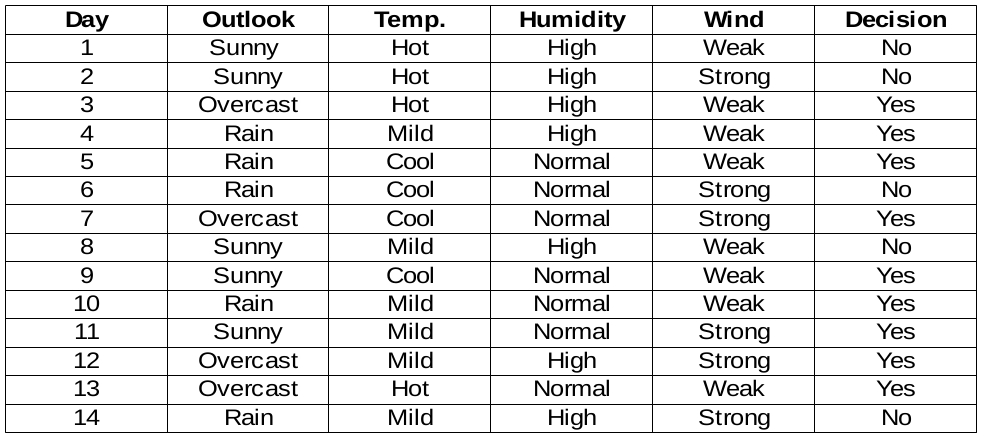
We need to find the most important feature w.r.t target columns to choose the node to split data in this data set.
Chi-Square Calculations
Now here’s how we calculate the chi-square values for various features.
Humidity Feature
There are two types of classes present in humidity columns, which are high and normal. Now we will calculate the chi_square values for them.
| yes | No | Total | Expected | Chi-square Yes | Chi-square No | |
| High | 3 | 4 | 7 | 3.5 | 0.267 | 0.267 |
| low | 6 | 1 | 7 | 3.5 | 1.336 | 1.336 |
For each row, the total column is the sum of yes and no decisions. Half of the total column is called Expected values because there are 2 classes in the decision. It is easy to calculate the chi-squared values based on this table.
For example,
chi-square yes for high humidity is √(( 3– 3.5)2 / 3.5) = 0.267
whereas actual is 3 and expected is 3.5.
So, the chi-square value of the humidity feature is
= 0.267 + 0.267 + 1.336 + 1.336
= 3.207
Now, we will find chi-square values for other features also. The feature having the maximum chi-square value will be the decision point. What about the wind feature?
Wind Feature
There are two types of classes present in wind columns, which are weak and strong. The following table is the below table.
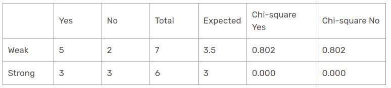
Herein, the chi-square test value of the wind feature is
= 0.802 + 0.802 + 0 + 0
= 1.604
This is less value than the chi-square value of humidity as well. What about the temperature feature?
Temperature Feature
There are three types of classes present in temperature columns, which are hot, cool, and mild. The following table is the below table.
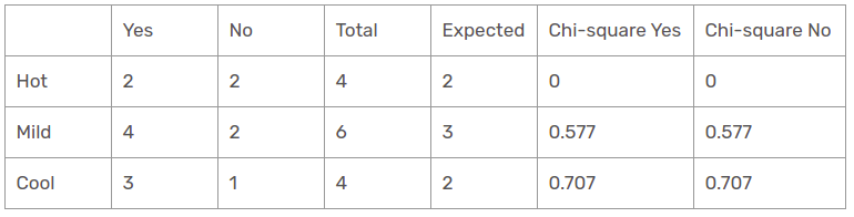
Herein, the chi-square test value of the temperature feature is
= 0 + 0 + 0.577 + 0.577 + 0.707 + 0.707
= 2.569
This is less value than the chi-square value of humidity and greater than the chi_square value of wind as well. What about the outlook feature?
Outlook Feature
There are three types of classes present in temperature columns, which are sunny, rain, and overcast. The following table is the below table.
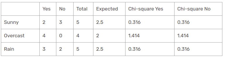
Herein, the chi-square test value of the outlook feature is
= 0.316 + 0.316 + 1.414 + 1.414 + 0.316 + 0.316
= 4.092
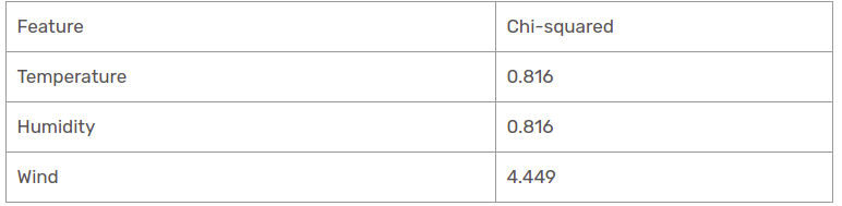
We have calculated the chi-square values of all features. Let’s see them all at one table.
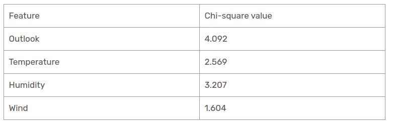
As seen, the outlook column has the most elevated and highest chi-square value. This implies that it is the main component feature. Along with these values, we will put this feature to the root node.
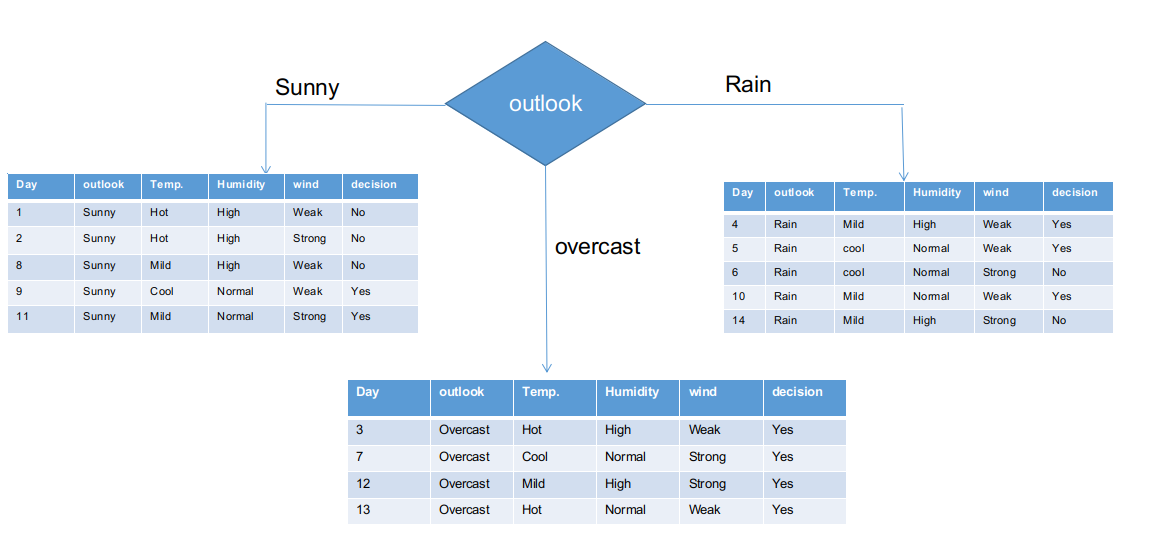
We’ve separated the raw information based on the outlook classes in the illustration above. For instance, the overcast branch simply has a yes decision in the sub informational dataset. This implies that the CHAID tree returns YES if the outlook is overcast.
Both sunny and rain branches have yes and no decisions. We will now apply chi-square tests for these sub informational datasets.
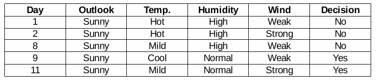
Outlook Sunny branch
This branch has 5 examples. Presently, we search for the most predominant feature. By The Way, we will disregard the outlook feature now since they are altogether the same. At the end of the day, we will find out the most predominant columns among temperature, humidity, and wind.
Humidity Feature for When the Outlook is Sunny
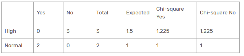
Chi-square value of humidity feature for sunny outlook is
= 1.225 + 1.225 + 1 + 1
= 4.449
Wind Feature for When the Outlook is Sunny
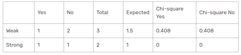
Chi-square value of wind feature for sunny outlook is
= 0.408 + 0.408 + 0 + 0
= 0.816
Temperature Feature for When the Outlook is Sunny
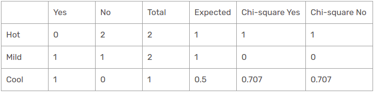
So, the chi-square value of temperature feature for sunny outlook is
= 1 + 1 + 0 + 0 + 0.707 + 0.707
= 3.414
We have found chi-square values for sunny is outlook. Let’s see them all at a table.
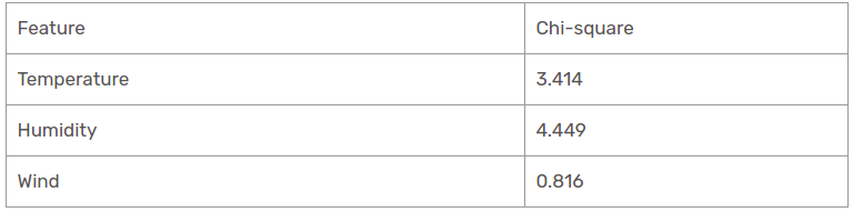
Presently, humidity is the most predominant feature for the sunny outlook branch. We will put this feature as a decision rule.
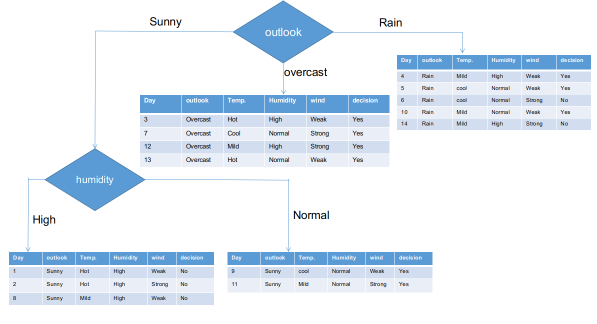
Presently, both humidity branches for sunny outlook have only one decision as delineated previously. CHAID tree will return NO for sunny outlook and high humidity and it will return YES for sunny outlook and normal humidity.
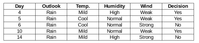
Rain Outlook branch
This branch actually has both yes and no decisions. We need to apply the chi-square test for this branch to find out an accurate decision. This branch has 5 distinct instances as demonstrated in the accompanying sub informational collection dataset. How about we find out the most predominant feature among temperature, humidity, and wind.
Wind Feature for Rain Outlook
There are two types of classes present in wind feature for rain outlook, which are weak and strong.
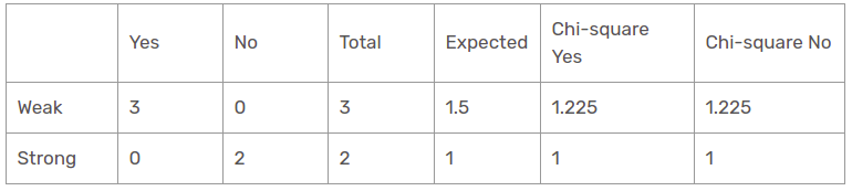
So, the chi-square value of wind feature for rain outlook is
= 1.225 + 1.225 + 1 + 1
= 4.449
Humidity Feature for Rain Outlook
There are two types of classes present in humidity feature for rain outlook, which are high and normal.
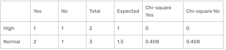
Chi-square value of humidity feature for rain outlook is
= 0 + 0 + 0.408 + 0.408
= 0.816
Temperature Feature for Rain Outlook
There are two types of classes present in temperature features for rain outlook, which are mild and cool.
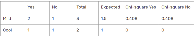
Chi-square value of temperature feature for rain outlook is
= 0 + 0 + 0.408 + 0.408
= 0.816
We have found all chi-square values for rain is outlook branch. Let’s see them all at a single table.
Thus, the wind feature is the victor for the rain is the outlook branch. Put this column in the connected branch and see the corresponding sub informational dataset.
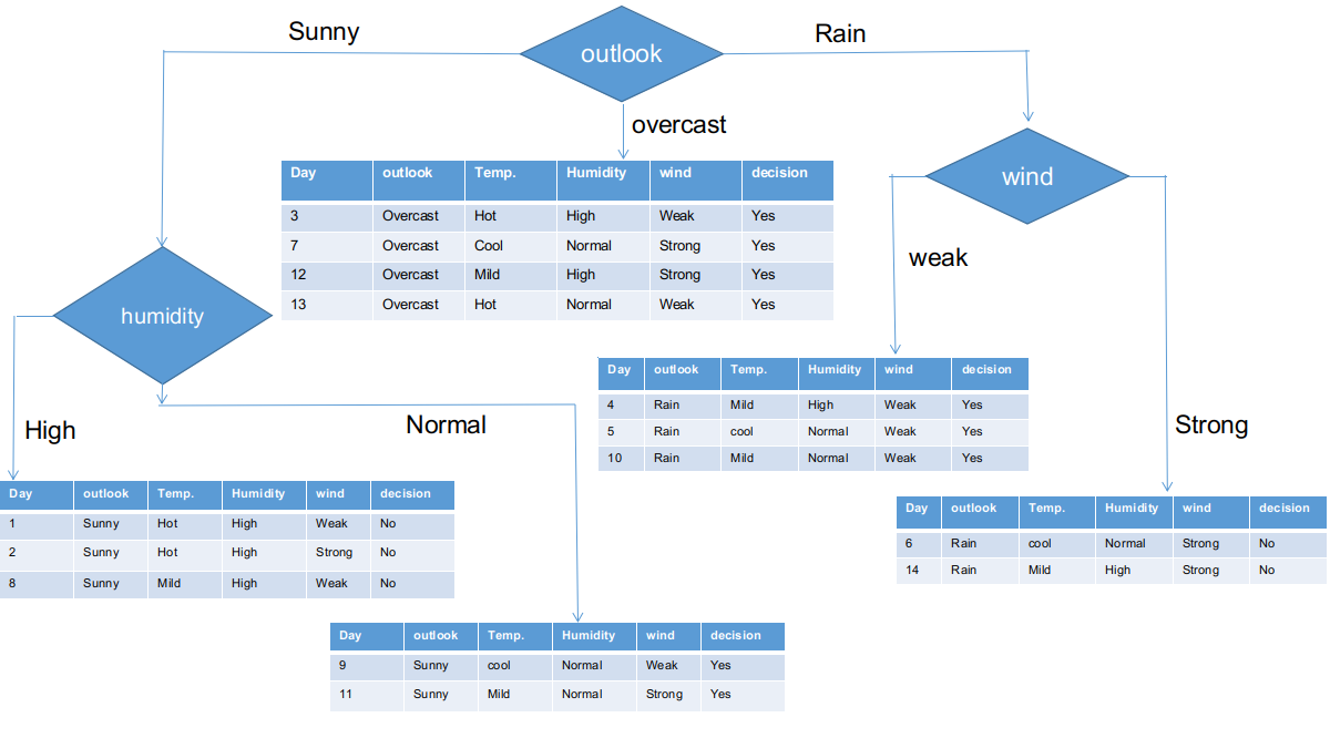
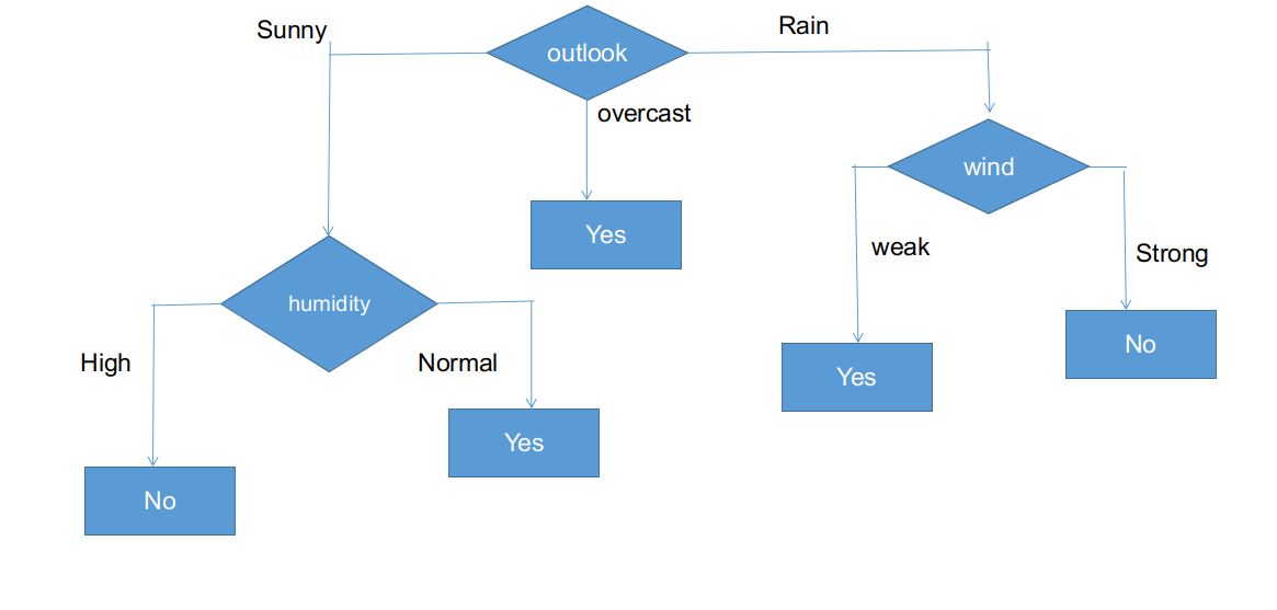
As seen, all branches have sub informational datasets having a single decision: yes or no. In this way, we can generate the CHAID tree as illustrated below.
Python Implementation of a Decision Tree Using CHAID
Python Code:
# Import the required library for CHAID
import chaid
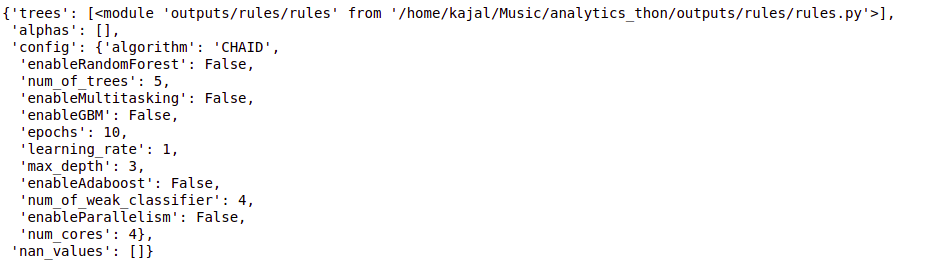
# Define the configuration for the CHAID algorithm
config = {"algorithm": "CHAID"}
# Fit the CHAID decision tree to the data
tree = chaid.fit(data, config)Tree
# Define a test instance for prediction
#test_instance = ['sunny','hot','high','weak','no']
test_instance = data.iloc[2]

# Display the test instance
test_instance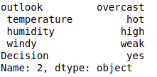
# Predict the outcome for the test instance using the CHAID decision tree
cb.predict(tree,test_instance)

output:- 'Yes'

#obj[0]: outlook, obj[1]: temperature, obj[2]: humidity, obj[3]: windy
# {"feature": "outlook", "instances": 14, "metric_value": 4.0933, "depth": 1}

# CHAID analysis function
def findDecision(obj):
          # Split based on the categorical variable "outlook"
          if obj[0] == 'rainy':
          # {"feature": " windy", "instances": 5, "metric_value": 4.4495, "depth": 2}
                  # Split based on the predictor variable "windy"
                  if obj[3] == 'weak':
                         return 'yes'
                  elif obj[3] == 'strong':
                         return 'no'
                  else:
                          return 'no'
          elif obj[0] == 'sunny':
           # {"feature": " humidity", "instances": 5, "metric_value": 4.4495, "depth": 2}
                 # Split based on the predictor variable "humidity"
                 if obj[2] == 'high':
                        return 'no'
                 elif obj[2] == 'normal':
                         return 'yes'
                 else:
                         return 'yes'
         elif obj[0] == 'overcast':
                      # Split based on the predictor variable "outlook"
                      return 'yes'
         else:
                    return 'yes'
Conclusion
Thus, we have created a CHAID decision tree from scratch to end in this post. CHAID uses a chi-square measurement metric to find out the most important feature and apply this recursively until sub informational datasets have a single decision. Even though this is a legacy decision tree algorithm, it is as yet the same process for classification problems.
Key Takeaways
- Decision trees are highly accurate and easy-to-understand predictive models used in supervised learning, making them popular choices for data analysis tasks.
- Various algorithms, including CART, ID3, C4.5, and CHAID, are available for constructing decision trees, each employing different criteria for node splitting.
- The CHAID algorithm uses the chi-square metric to determine the most important features and recursively splits the dataset until sub-groups have a single decision.
- Interpreting CHAID decision trees involves analyzing split decisions based on categorical variables such as outlook, temperature, humidity, and windy conditions.
- Understanding CHAID decision trees is valuable for data analysts and data scientists working on classification problems, as it offers insights into the decision-making process and the importance of different predictor variables.
Frequently Asked Questions
Q1. What is the difference between regression and CHAID?
A. The main difference between regression and CHAID lies in their approach to handling data types and the nature of the analysis. Regression is primarily used for predicting continuous outcome variables and finding the best split based on numerical data, while CHAID analysis is specifically designed for categorical data. CHAID, which stands for “Chi-square Automatic Interaction Detector,” employs the chi-square statistic and F-test to identify the best splits in categorical variables, making it well-suited for analyzing categorical data and determining the most significant predictors in a dataset.
Q2. How do you interpret the results of a CHAID decision tree analysis?
A. Interpreting the results of a CHAID decision tree analysis involves evaluating the significance of predictors using p-values, identifying the response variable, ensuring a large sample size, and potentially applying logistic regression for additional analysis.
Q3. What are the advantages and disadvantages of using a CHAID decision tree in data analysis?
A. The advantages of using a CHAID decision tree in data analysis include its versatility for both classification and regression tasks in data science. It can handle categorical and continuous independent variables, providing insights into respondent behavior.
Disadvantages may include potential overfitting, particularly with complex datasets, and the inability to capture interactions between variables, which may limit its usefulness in regression analysis.
The media shown in this article are not owned by Analytics Vidhya and are used at the Author’s discretion.
Hi, I am Kajal Kumari. have completed my Master’s from IIT(ISM) Dhanbad in Computer Science & Engineering. As of now, I am working as Machine Learning Engineer in Hyderabad.
hope that you have enjoyed the article. If you like it, share it with your friends also. Please feel free to comment if you have any thoughts that can improve my article writing.
If you want to read my previous blogs, you can read Previous Data Science Blog posts here. Connect with me


Good job👍 It seems you have good command on coding skills. Keep posting such articles ❤
That's a very good explanation of CHAID with and example. I am wondering if CHAID can be used for a dataset with a column which as continuous values. For example what if the temperature column has the actual temperature values( 23, 14, 17, 22, 09 etc.). What approach do you suggest to use in order to use CHAID to build a decision tree.