Introduction
Order statistics are a very useful concept in statistical sciences. They have a wide range of applications including modeling auctions, car races, and insurance policies, optimizing production processes, estimating parameters of distributions, et al. Through this article, we’ll understand the idea of order statistics. We’ll first understand its meaning and gradually proceed to its distribution, eventually covering more advanced concepts.
Suppose we have a set of random variables X1, X2, …, Xn, which are independent and identically distributed (i.i.d). By independence, we mean that the value taken by a random variable is not influenced by the values taken by other random variables. By identical distribution, we mean that the probability density function (PDF) (or equivalently, the Cumulative distribution function, CDF) for the random variables is the same. The kth order statistic for this set of random variables is defined as the kth smallest value of the sample.
To better understand this concept, we’ll take 5 random variables X1, X2, X3, X4, X5. We’ll observe a random realization/outcome from the distribution of each of these random variables. Suppose we get the following values:

The kth order statistic for this experiment is the kth smallest value from the set {4, 2, 7, 11, 5}. So, the 1st order statistic is 2 (smallest value), the 2nd order statistic is 4 (next smallest), and so on. The 5th order statistic is the fifth smallest value (the largest value), which is 11. We repeat this process many times i.e., we draw samples from the distribution of each of these i.i.d random variables, & find the kth smallest value for each set of observations. The probability distribution of these values gives the distribution of the kth order statistics.
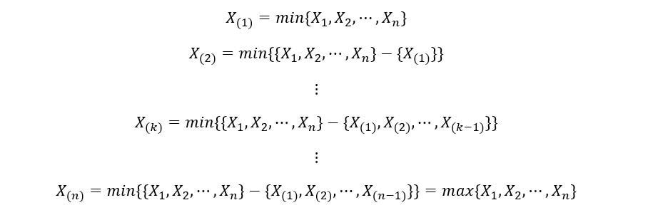
In general, if we arrange random variables X1, X2, …, Xn in ascending order, then the kth order statistic is shown as:

The general notation of the kth order statistic is X(k). Note X(k) is different from Xk. Xk is the kth random variable from our set, whereas X(k) is the kth order statistic from our set. X(k) takes the value of Xk if Xk is the kth random variable when the realizations are arranged in ascending order.
The 1st order statistic X(1) is the set of the minimum values from the realization of the set of ‘n’ random variables. The nth order statistic X(n) is the set of the maximum values (nth minimum values) from the realization of the set of ‘n’ random variables. They can be expressed as:
Distribution of Order Statistics
We’ll now try to find out the distribution of order statistics. We’ll first describe the distribution of the nth order statistic, then the 1st order statistic & finally the kth order statistic in general.
A) Distribution of the nth Order Statistic:
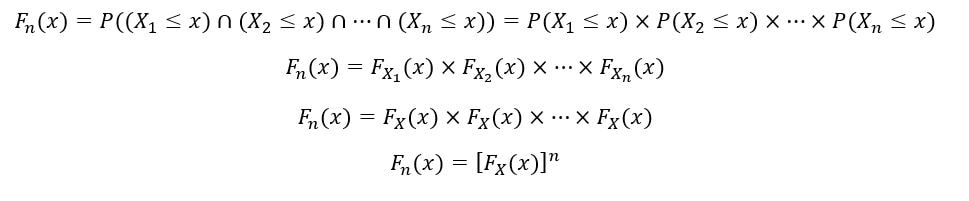
Let the probability density function (PDF) & cumulative distribution function (CDF) our random variables be fx(x), and Fx(x) respectively. By definition of CDF,

Since our random variables are identically distributed, they have the same PDF fx(x) & CDF Fx(x). We’ll now calculate the CDF of nth order statistic (Fn(x)) as follows:

The random variables X1, X2, …, Xn are also independent. Therefore, by property of independence,
The PDF of the nth order statistic (fn(x)) is calculated as follows:
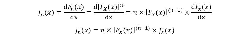
Thus, the expression for the PDF & CDF of nth order statistic has been obtained.
B) Distribution of the 1st Order Statistic:
The CDF of a random variable can also be calculated as the one minus the probability that the random variable X takes a value more than or equal to x. Mathematically,

We’ll determine the CDF of 1st order statistic (F1(x)) as follows:
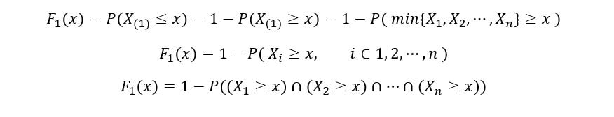
Once again, using the property of independence of random variables,
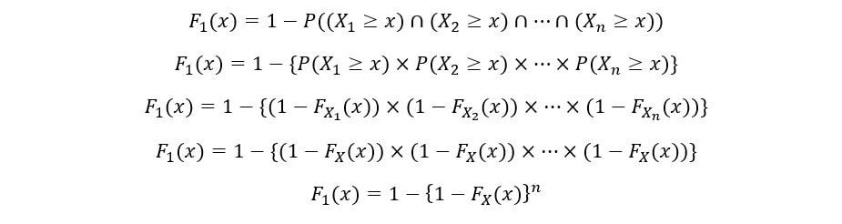
The PDF of the 1st order statistic (f1(x)) is calculated as follows:
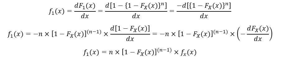
Thus, the expression for PDF & CDF of 1st order statistic has been obtained.
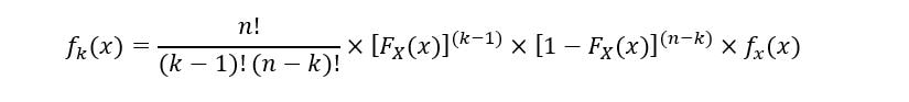
C) Distribution of the kth Order Statistic:
For kth order statistic, in general, the following equation describes its CDF (Fk(x)):

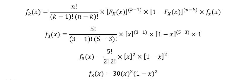
The PDF of kth order statistic (fk(x)) is expressed as:
To avoid confusion, we’ll use geometric proof to understand the equation. As discussed before, the set of random variables have the same PDF (fX(x)). The following graph shows a sample PDF with the kth order statistic obtained from random sampling:
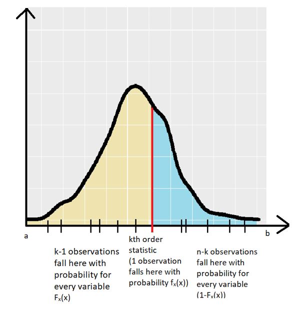
So, the PDF of the random variables fX(x) is defined between the interval [a,b]. The kth order statistic for a random sample is shown by the red line. The other variable realizations (for the random sample) are shown by the small black lines on the x-axis.
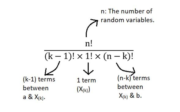
There are exactly (k – 1) random variable observations that fall in the yellow region of the graph (the region between a & kth order statistic). The probability that a particular observation falls in this region is given by the CDF of the random variables (FX(x)). But we are aware that (k – 1) observations did fall in the region, which gives us the term (by independence) (FX(x))(k – 1).
There are exactly (n – k) random variable observations that fall in the blue region of the graph (the region between kth order statistic & b). The probability that a particular observation falls in this region is given by the 1 – CDF of the random variables (1– FX(x)). But we are aware that (n – k) observations did fall in the region, which gives us the term (by independence) (1–FX(x))(n – k).
Finally, exactly 1 observation falls exactly at the kth order statistic with probability fX(x). Thus, the product of the 3 terms gives us an idea of the geometric meaning of the equation for PDF of the kth order statistic. But where does the factorial term come from? The above scenario just showed one of the many orderings. There can be many such combinations. The total number of such combinations is shown as follows:
Thus, the product of all of these terms gives us the general distribution of the kth order statistic.
Useful Functions of Order Statistics
Order statistics give rise to various useful functions. Among them, the notable ones include sample range and sample median.
1) Sample range: It is defined as the difference between the largest and smallest value. It is expressed as follows:

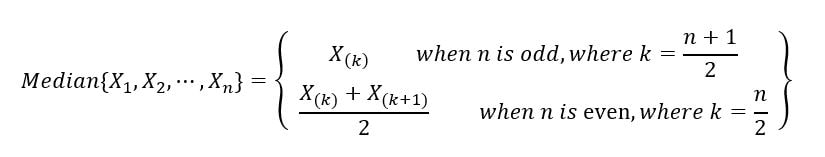
2) Sample median: The sample median divides the random sample (realizations from the set of random variables) into two halves, one that contains samples with lower values, and the other that contains the samples with higher values. It’s like the middle/central order statistic. It is mathematically defined as:
Joint PDF of Order Statistics
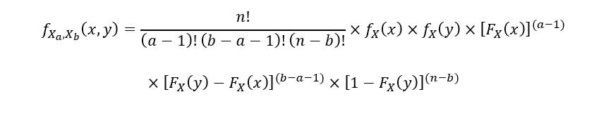
A joint probability density function can help us better understand the relationship between two random variables (two order statistics
in our case). The joint PDF for any 2 order statistics X(a) & X(b), such that 1 ≤ a ≤ b ≤ n is given by the following equation:
Example
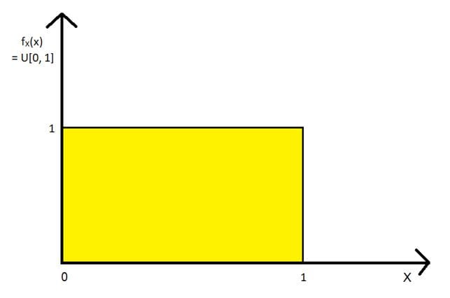
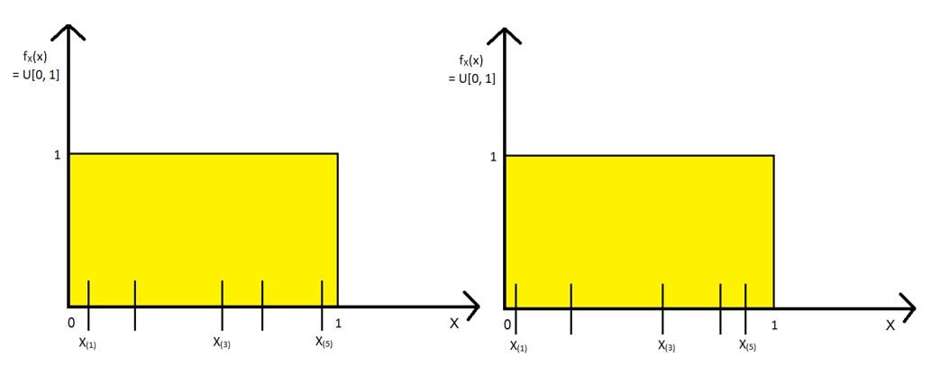
We’ll use a very simple example to illustrate the distribution of order statistics- the standard uniform distribution (U[0, 1] distribution). We’ll take 5 random variables X1, X2, X3, X4, X5, all having the U[0, 1] distribution. For this set of random variables, we’ll calculate & plot the 1st, 3rd (the sample median) & 5th (nth) order statistics. The following figure shows the U[0, 1] distribution:
We’ll draw random samples as follows and find the 1st, 3rd & 5th order statistic for each sample. Two of the samples are shown below:
The PDF & CDF of standard uniform distribution is given as:

We’ll use this information and calculate X(1), X(3) & X(5) using the formulas we derived. We’ll take the case only when x is between 0 & 1 (for other cases, the order statistic is zero as PDF is zero).
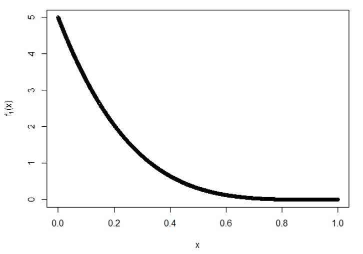
A) For 1st order statistic:

Plot for f1(x):
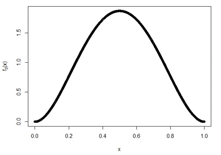
B) For 3rd order statistic:
Plot for f5(x):
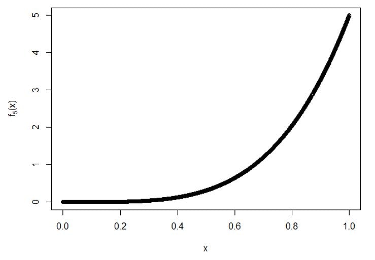
C) For 5th order statistic:

Plot for f5(x):
Conclusion
Thus, we’ve explored the concepts of order statistics thoroughly. A wide range of physical processes can be modeled through order statistics, by exploiting their properties, particularly their distributions.
The media shown in this article are not owned by Analytics Vidhya and is used at the Author’s discretion.


You said one observation fall in red line ok. But fx(x) is not thats observations probability. Because this is PDF!!
Its was really simplified and easy to understand, great job