Neural network and hyperparameter optimization using Talos

This article was published as a part of the Data Science Blogathon

In terms of ML, what neural network means?

A neural network is composed of a network of artificial neurons or nodes. These artificial networks may be used for predictive modelling or different decision-making applications. Different weights are assigned to different nodes and it is iterated over and over to obtain the best network of nodes for the given problem statement.

It consists of three layers of nodes.

• Input layer: The number of nodes depends upon the number of input variable or exogenous variables
• Output layer: The number of nodes depends on the output. If it is a classification model, the number of output would be equal to different classes present in the dependent variable
• Hidden layer: It can contain multiple to single layer of nodes with each node having some function by taking input from the previous layer to sending output to the next layer

Importing necessary libraries

Here we are using the KerasRegressor package to perform regression. To read more about the package click here

Below is the list of files to be imported from KerasRegressor:

#packages for neural networking
from keras.callbacks import ModelCheckpoint
from keras.models import Sequential
from keras.layers import Dense, Activation, Flatten
from keras.wrappers.scikit_learn import KerasRegressor
from keras.optimizers import Adam
from keras.optimizers import SGD
from keras.activations import relu, elu
import talos

Parameters used in KerasRegressor

Activation

Activation is a function that is implemented on nodes. There are primarily three input and three output activation functions:

1. Input function: Rectified linear activation (relu): It is the most commonly used activation function and calculated as max(0,0,x) which means if x is negative then the function will return 0 otherwise x.

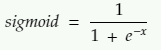
2. Input function: Sigmoid: It is also known as the logistic function. It takes any value as input and returns in the range of 0 to 1. It is calculated as

3. Input function: Tanh: It is similar to the sigmoid function but it ranges from -1 to 1 and calculated as

4. Output function: Linear: It is default and it does not change any input data used for regression

5. Output function: Sigmoid: It is the same as input activation and used for Binary classification since the output is 1 or 0

6. Output function: Softmax: It used for multi-classification and calculated as

If you are still unsure about which activation function to use try to use a few and tune according to the need.

Units

This is used to define the number of nodes present in a layer. There is no specified logic in what should be the number of nodes but many data scientists prefer to keep it in the power of 2.

    ###################### Following code add a layer of neural network with ################
    ###################### node = 64 and activation = relu ##################################
    regressor.add(Dense(units=64, activation = 'relu'))

Adding layers

To add a layer, just use the ‘REGRESSOR.ADD()’ function and the required parameters. The only difference would be in adding the input and output layer. In the input layer, we add a parameter ‘input_dim’ to define the number of exogenous variables in addition to defining the number of nodes. Generally, we keep the value of ‘input_dim’ equivalent to ‘units’ to take all the input variables in the raw and unhindered state for our first layer.

For the last, output layer we need to define the units as 1 and activation = ‘linear’ (which is the default) for regression. Similarly. for binary classification we need to set the activation as sigmoid. The below example shows the addition of one input layer, three hidden layers, and one output layer

    ################## Addition of one input layer with 100 exogeneous variables ###########
    regressor.add(Dense(units=100, input_dim=100, activation = 'relu'))
    ################## Addition of 3 hidden layers #########################################
    regressor.add(Dense(units=64, activation = 'relu'))
    regressor.add(Dense(units=8, activation = 'relu'))
    regressor.add(Dense(units=4, activation = 'relu'))
    ################## Addition of one output layer with one node ##########################
    regressor.add(Dense(units=1))

If you want to have more additional hidden layers just add “REGRESSOR.ADD()” between the desired layers. There is no upper limit on the number of hidden layers

Optimizer

Optimizers are algorithm or method that changes the learning rate and weights of a neural network to reduce the losses. There are 4 major optimizers used in the neural network

1. Adam (Adaptive Momentum Estimation): This is considered to be the best optimizer as it takes lesser time and is more efficient

2. Gradient descent: It is the most used and simplest optimizer. it calculates a way in which weight is altered through backpropagation. It has a few disadvantages such as it take a large amount of time and it can be stuck on local minima

3. SGD (Stochastic Gradient Descent): It is faster than Gradient descent optimizer as it updates the model parameter more frequently compared to Gradient descent which does only one time. It has few disadvantages such as it gives high variance in model parameter due to frequent update and it may end up at local minima

4. SGD with Momentum: It was invented to handle the disadvantage of SGD by reducing the fluctuation

Other optimizers one could try like AdaDelta, Adagrad, Nesterov Accelerated Gradient(NAG), Mini Batch Stochastic Gradient Descent (MB-SGD), RMSprop. These can be discussed later on.

Learning rate

It ranges from 0 to 1. The weight of nodes is altered in every iteration, learning rate represents the amount that the weights are updated during training of the model. A high learning rate could overfit the model and a low learning rate could give an inferior model.

Loss function

The neural network tends to minimize the error as much as it can, for that to happen neural network uses a metric to quantify the error which is referred to as the Loss function. After each iteration neural network calculates the loss function and restructures the weights to minimize the error. The high value of the loss metric would push the model harder to adjust the weights of the neuron. Few loss functions:

1. Mean Squared Error(MSE): It is mostly used in regression and it is calculated by calculating the mean of the squared differences of the prediction and the actual values. This metric penalizes the model even for a small error.

2. Mean Squared Log Error(MSLE): It is used in place of MSE to penalize the model lesser by taking the log of error instead of taking just the difference of prediction and the actual values.

3. Mean Absolute Error(MAE): It is calculated by calculating the mean of the absolute difference of prediction and the actual values. Make sure to scale the variable first before using this function as it can be highly susceptible to outliers.

4. Cross-Entropy: It is used in Binary and multi-class classification and it is calculated by taking the difference of average actual and predicted probability of the defined class.

5. Hinge Loss: It is used in Binary and multi-class classification and it penalizes the model more if there is a difference between the actual and predicted probability.

One can use and experiment with any of these loss functions as per their need or can include them in hyperparameter optimization to get the best loss contributing to a better model. How to perform hyperparameter optimization is explained later in this article.

Metrics

It is used to evaluate the model. We can use multiple metrics for evaluation. Since we are using regression we would be using mean average error and accuracy.

    ################### Adam optimizer with learning rate = 0.01 ###########################
    opt = Adam(lr = 0.01)
    ################### loss function as mean squared error and ############################
    ################### evaluation metric as mae and accuracy ##############################
    regressor.compile(optimizer=opt, loss='mean_squared_error',  metrics=['mae','accuracy'])

Batch size

It is the size of the dataset used as a training set in one iteration. To use the whole dataset keep batch size equal to the number of the dataset

Epoch

One epoch refers to one learning cycle of an entire dataset. Neural network stops the iteration when there isn’t any change in the loss which can sometimes lead to overfitting of the model. Hence, to avoid overfitting one can introduce epoch.

def build_regressor():
    ############### Sequential function is to initiate the layers in the Neural model ##########
    regressor = Sequential()
    regressor.add(Dense(units=165, input_dim=165, activation = 'relu'))
    regressor.add(Dense(units=64, activation = 'relu'))
    regressor.add(Dense(units=8, activation = 'relu'))
    regressor.add(Dense(units=4, activation = 'relu'))
    regressor.add(Dense(units=1))
    opt = Adam(lr = 0.01)
    regressor.compile(optimizer=opt, loss='mean_squared_error',  metrics=['mae','accuracy'])
    return regressor

regressor = KerasRegressor(build_fn=build_regressor, batch_size=1000,epochs=60, verbose = False)
results=regressor.fit(X_train,y_train)

loss_train = results.history['loss']
epochs = range(0,len(loss_train))
plt.plot(epochs, loss_train, 'g', label='Training loss')
plt.xlabel('Epochs')
plt.ylabel('Loss')
plt.legend()
plt.show()

The above graph shows training loss wrt the number of epochs. Initially, the loss was high but after model learning at each epoch, it gradually decreased. Notice after 10 epoch it’s almost a straight line and would have continued till epoch = 100 or till the number of iterations specified and there wouldn’t be any significant difference in the loss metric and eval metric between 20 epochs to 100 epochs but overfitting the model at each epoch.

Hyperparameter Optimization

For hyperparameter optimization select the parameters which you want to tune and what values you would like the parameter to choose from. Remember higher the size of parameters, the longer it would take the model to tune.

Pro tip: Iterate few parameters by yourself to choose which is giving better results

In this section Talos package is used for hyperparameter tuning. To read more about the package click here

Parameter fixed by running few iterations:

• activation = relu
• number of hidden layer = 3
• optimizer = adam
• loss = mean_squared_error
• epochs = 100

Parameter used for optimization:

• number of neuron = [4, 8, 12, 24, 48,64]
• batch_size = [1000, 2000, 7000]

############### p contains the dictionary of parameter to be tuned ###########################
p = {'first_neuron': [4, 8, 12, 24, 48,64],
    'second_neuron': [4, 8, 12, 24, 48,64],
    'third_neuron': [4, 8, 12, 24, 48,64],
    'activation': ['relu'],
    'batch_size': [1000, 2000, 7000]
}
################ add input parameters to the function ########################################
def outage(x_train, y_train, x_val, y_val, params):
    ########## replace the hyperparameter inputs with references to params dictionary ########
    model = Sequential()
    ################### Input layer ##########################################################
    model.add(Dense(100, input_dim=100, activation=params['activation']))
    #################### Introducing 3 hidden layers #########################################
    model.add(Dense(params['first_neuron'], activation=params['activation']))
    model.add(Dense(params['second_neuron'], activation=params['activation']))
    model.add(Dense(params['third_neuron'], activation=params['activation']))
    #################### Output layer with activation = linear (default) ####################
    model.add(Dense(1))
    #################### Defining loss function, optimizer and accuracy #####################
    model.compile(loss='mean_squared_error', optimizer='adam', metrics=['accuracy'])
    ################### make sure history object is returned by model.fit() #################
    out = model.fit(x=x_train, 
                    y=y_train,
                    validation_data=[x_val, y_val],
                    epochs=100,
                    batch_size=params['batch_size'],
                    verbose= False)
    ################### return the output model #############################################
    return out, model
    
####################### Talos hyperparameter ################################################
t = talos.Scan(x=x_train, y=y_train, 
              params=p, model=outage, experiment_name='neural')
###################### This code will deploy the model as a zip file ########################
talos.Deploy(scan_object=t, model_name='neural_final', metric='accuracy')
###################### This will extract the deployed zip file and can be used for ##########
###################### Predictions ##########################################################
final_model= talos.Restore('neural_final.zip')
######################### make predictions with the model ###################################
y_pred  = final_model.model.predict(X_test)

Conclusion

In this article, you learned what is the basic parameter and how it impacts the neural network and how to implement a neural network for performing regression using Keras. Also, you learned how to use Talos for Hyperparameter Optimization. These will help in creating a standard version of hyperparameter optimization of neural networks.

If you have any doubts or suggestion reply in the comments or connect with me on LinkedIn

The media shown in this article are not owned by Analytics Vidhya and is used at the Author’s discretion.