This article was published as a part of the Data Science Blogathon
Hello readers. This is Part 2 in the series of A Comprehensive tutorial on Deep learning. If you haven’t read the first part, you can read about it here:
A comprehensive tutorial on Deep Learning – Part 1 | Sion
In the first part we discussed the following topics:
In this article, we will continue the discussion and introduce Artificial Neural Networks(ANN)
1) Artificial Neural Networks
2) 2 Layered Neural Network
3) What to expect in the next article
4) Endnotes
This is another name for Deep Neural network or Deep Learning.
What neural network essentially means is we take logistic regression and repeat it multiple times. In a normal logistic regression, we have an input layer and an output layer. But in the case of a Neural Network, there is at least one hidden layer of regression between these input and output layers.
Well of course there is no specific amount of layers to classify a neural network as deep. The term “Deep” is quite frankly relative to every problem. The correct question we can ask is “How much deep?”. For example, the answer to “How deep is your swimming pool?” can be answered in multiple ways. It could be 2 meters deep or 10 meters deep, but it has “depth”. Same with our neural network, it can have 2 hidden layers or “thousands” hidden layers(yes you heard that correctly).
So I’d like to just stick with the question of “How much deep?” for the time being.
They are called hidden because they do not see the original inputs( the training set ). For example, let’s say you have a NN with an input layer, one hidden layer, and an output layer. When asked how many layers your NN has, your answer should be “It has 2 layers”, because while computation the initial, or the input layer, is ignored.
Let me help visualize how a 2 layer Neural network looks like:
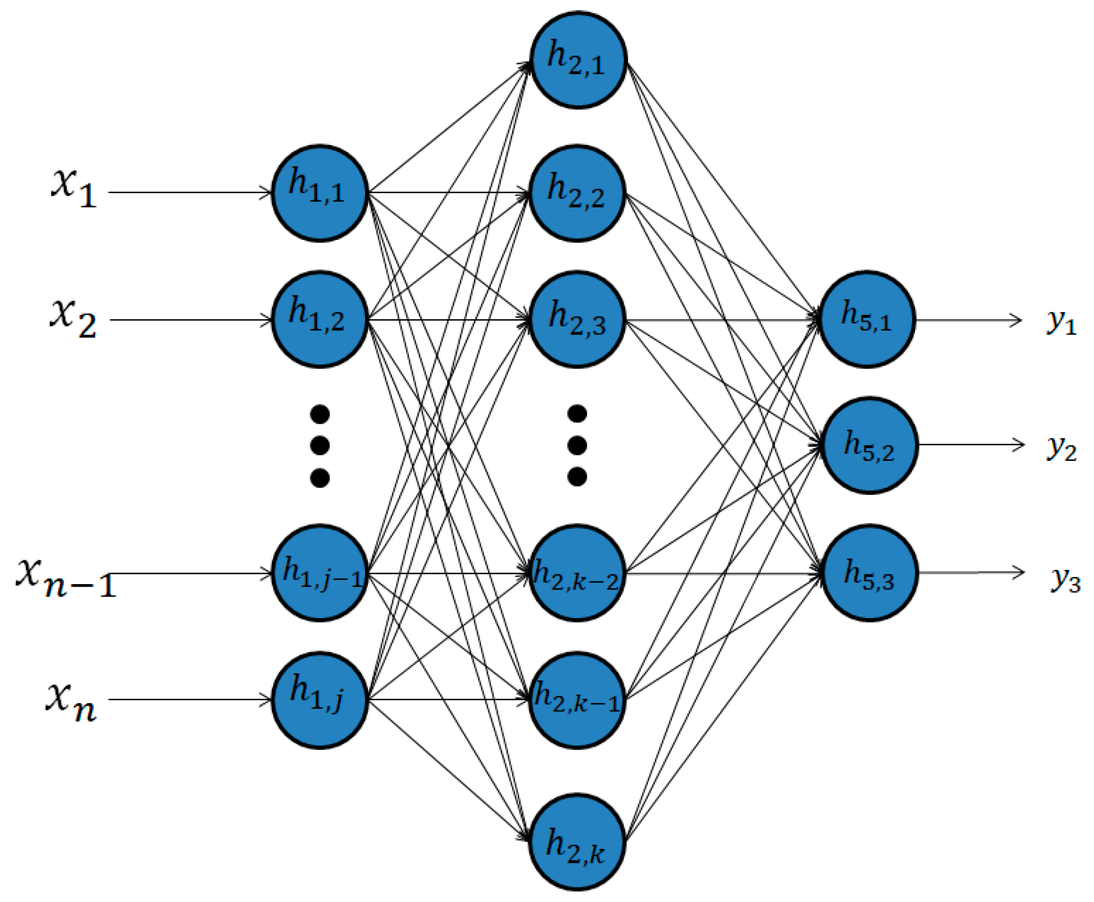
Step by step we shall understand this image.
1) As you can see here we have a 2 Layered Artificial Neural Network. A Neural network was created to mimic the biological neuron of the human brain. In our ANN we have a “k” number of nodes. The number of nodes is a hyperparameter, which essentially means that the amount is configured by the practitioner making the model.
2) The inputs and outputs layers do not change. We have “n” input features and 3 possible outcomes.
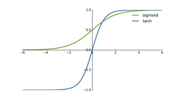
3) Unlike Logistic regression, neural networks use the tanh function as their activation function instead of the sigmoid function which you are quite familiar with. The reason is that the mean of its output is closer to 0 which makes the more centered for input to the next layer. tanh function can cause an increase in non-linearity which makes our model learn better.
4) In normal logistic regression: Input => Output.
Whereas in a Neural network: Input => Hidden Layer => Output. The hidden layer can be imagined as the output of part 1 and input of part 2 of our ANN.
Now let us have a more practical approach to a 2 Layered Neural Network.
(Important Note: We shall continue where we left off in the previous article. I’m not going to waste your time and mine by loading the dataset again and preparing it. The link to the Part 1 of this series is given above.)
Our training set has 348 samples, thus x(348). In logistic regression, we initialized the bias at 0 and weights at 0.01. But this time we shall initialize the weights randomly because if we initialize them with 0, all the neurons in the 1st layer will be computing the same things as the other neurons. Thus we shall initialize randomly. Also, these initial weights should be small because if they are large in the beginning, they shall cause the inputs to tanh to be large, causing the gradients to be close to 0, making the optimization algorithm slow.
Biases can be made 0 initially.
# intialize parameters and layer sizes
def initialize_parameters_and_layer_sizes_NN(x_train, y_train):
    parameters = {"weight1": np.random.randn(3,x_train.shape[0]) * 0.1,
                  "bias1": np.zeros((3,1)),
                  "weight2": np.random.randn(y_train.shape[0],3) * 0.1,
                  "bias2": np.zeros((y_train.shape[0],1))}
    return parameters
The forward propagation is almost the same as we used in Logistic regression. The only difference here is that we use the tanh function and do all the processes twice. The tanh function is included in the Numpy module.
def forward_propagation_NN(x_train, parameters):

    Z1 = np.dot(parameters["weight1"],x_train) +parameters["bias1"]
    A1 = np.tanh(Z1)
    Z2 = np.dot(parameters["weight2"],A1) + parameters["bias2"]
    A2 = sigmoid(Z2)

    cache = {"Z1": Z1,
             "A1": A1,
             "Z2": Z2,
             "A2": A2}

    return A2, cache
The loss and cost functions are the same as the logistic regression.
The cross-entropy loss:
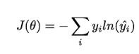
# Compute cost
def compute_cost_NN(A2, Y, parameters):
    logprobs = np.multiply(np.log(A2),Y)
    cost = -np.sum(logprobs)/Y.shape[1]
    return cost
Backward propagation is essentially the derivative. This is a very extensive and crucial topic which deserves an article of its own. Be sure to check out my future articles for a tutorial on Backpropagation. Let us write the code:
# Backward Propagation
def backward_propagation_NN(parameters, cache, X, Y):

    dZ2 = cache["A2"]-Y
    dW2 = np.dot(dZ2,cache["A1"].T)/X.shape[1]
    db2 = np.sum(dZ2,axis =1,keepdims=True)/X.shape[1]
    dZ1 = np.dot(parameters["weight2"].T,dZ2)*(1 - np.power(cache["A1"], 2))
    dW1 = np.dot(dZ1,X.T)/X.shape[1]
    db1 = np.sum(dZ1,axis =1,keepdims=True)/X.shape[1]
    grads = {"dweight1": dW1,
             "dbias1": db1,
             "dweight2": dW2,
             "dbias2": db2}
    return grads
The updating of the Parameters is also the same as Logistic regression. This is the reason why you should read Part 1 of this series. We shall use the Logistic regression several times since it is the building block of an Artificial Neural Network.
# update parameters
def update_parameters_NN(parameters, grads, learning_rate = 0.01):
    parameters = {"weight1": parameters["weight1"]-learning_rate*grads["dweight1"],
                  "bias1": parameters["bias1"]-learning_rate*grads["dbias1"],
                  "weight2": parameters["weight2"]-learning_rate*grads["dweight2"],
                  "bias2": parameters["bias2"]-learning_rate*grads["dbias2"]}

    return parameters
Now we create a function for prediction:
# prediction
def predict_NN(parameters,x_test):
    # x_test is a input for forward propagation
    A2, cache = forward_propagation_NN(x_test,parameters)
    Y_prediction = np.zeros((1,x_test.shape[1]))
    # if z is bigger than 0.5, our prediction is sign one (y_head=1),
    # if z is smaller than 0.5, our prediction is sign zero (y_head=0),
    for i in range(A2.shape[1]):
        if A2[0,i]<= 0.5:
            Y_prediction[0,i] = 0
        else:
            Y_prediction[0,i] = 1

    return Y_prediction
Now time to put all of them together and see the magic happen:
# 2 - Layer neural network
def two_layer_neural_network(x_train, y_train,x_test,y_test, num_iterations):
    cost_list = []
    index_list = []
    #initialize parameters and layer sizes
    parameters = initialize_parameters_and_layer_sizes_NN(x_train, y_train)

    for i in range(0, num_iterations):
         # forward propagation
        A2, cache = forward_propagation_NN(x_train,parameters)
        # compute cost
        cost = compute_cost_NN(A2, y_train, parameters)
         # backward propagation
        grads = backward_propagation_NN(parameters, cache, x_train, y_train)
         # update parameters
        parameters = update_parameters_NN(parameters, grads)

        if i % 100 == 0:
            cost_list.append(cost)
            index_list.append(i)
            print ("Cost after iteration %i: %f" %(i, cost))
    plt.plot(index_list,cost_list)
    plt.xticks(index_list,rotation='vertical')
    plt.xlabel("Number of Iterarion")
    plt.ylabel("Cost")
    plt.show()

    # predict
    y_prediction_test = predict_NN(parameters,x_test)
    y_prediction_train = predict_NN(parameters,x_train)

    # Print train/test Errors
    print("train accuracy: {} %".format(100 - np.mean(np.abs(y_prediction_train - y_train)) * 100))
    print("test accuracy: {} %".format(100 - np.mean(np.abs(y_prediction_test - y_test)) * 100))
    return parameters

parameters = two_layer_neural_network(x_train, y_train,x_test,y_test, num_iterations=2500)
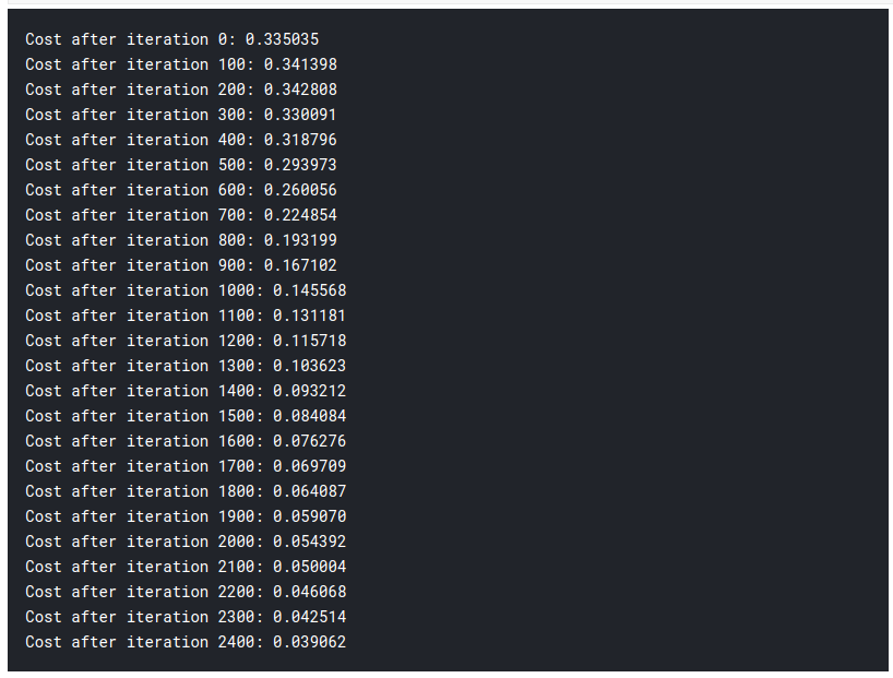
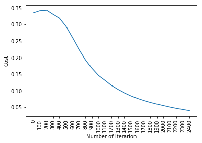
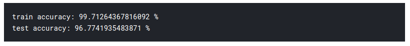
From the previous article, we had an accuracy of 92% after using the Logistic Regression. Thus you can see we have substantially higher accuracy by just adding an extra layer of Logistic regression. This is the reason why Neural Networks is one of the cutting-edge technologies nowadays.
In the next article, which I plan to publish shortly, we shall generalize the number of layers and build a model accordingly. In this article, we just used 1 hidden layer, and as you can see it performed really well. In the next article, we will create an L-layered Neural Network. Since it is really hectic to create functions and classes for each layer independently, we will use libraries like Keras and Pytorch for more efficient code.
Today you learned how to build your first neural network from scratch, congratulations! Although the same can be done with Keras with just a few lines of code, it’s always better to know what is happening under the hood. You can read the 3rd article in the link below after it’s published:
Sion | Author at Analytics Vidhya
Thank you and have a nice day, Cheers!!
The media shown in this article are not owned by Analytics Vidhya and are used at the Author’s discretion.
Lorem ipsum dolor sit amet, consectetur adipiscing elit,


