This article was published as a part of the Data Science Blogathon
Introduction
Let’s start the discussion with some questions. What is ensemble learning?
Ensemble learning is a learning technique in which multiple individual models combine to create a master model.
What is bagging and boosting? These two are the techniques or ways to implement ensemble models.
And what is a random forest? Random forest is an implementation of the bagging technique.
In this article, I will discuss the ensemble technique called boosting and a detailed explanation of Adaboost.
Table of contents
- Differences between bagging and boosting
- Understand Adaboost with data
- Final model
- Mathematical explanations
- Practical applications with Python
- Advantages and disadvantages
- References
1. Differences between bagging and boosting
The very first thing I want to cover here is what are the differences between bagging and boosting.
To be more specific let’s take one example from each set and I say the differences between random forest and Adaboost as the random forest is bagging technique and Adaboost is a boosting technique.
Both of these come under the family of ensemble learning.
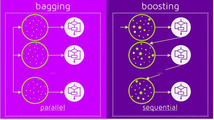
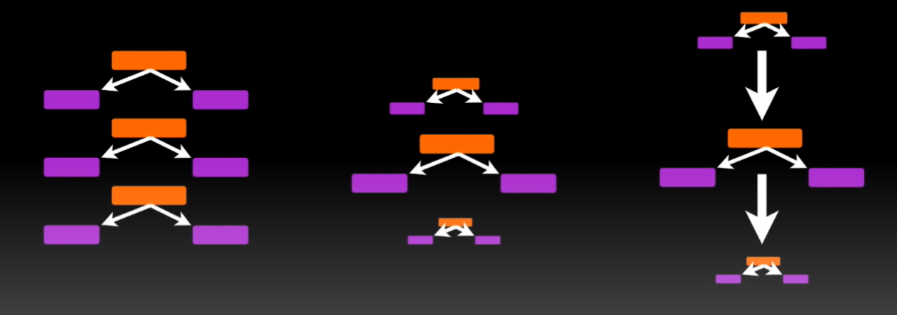
The first difference between random forest and Adaboost is random forest is a parallel learning process whereas Adaboost is a sequential learning process.
The meaning of this is in the random forest, the individual models or individual decision trees are built from the main data parallelly and independently of each other.
In the random forest, multiple trees are built from the same data parallelly and none of the trees is dependent on other trees. Hence this process is called a parallel process.
On the other hand, in the sequential process, one tree is dependent on the previous tree which means if there are multiple models implemented say ML model 1, ML model 2, ML model 3, and so on. Each of them has a process of ensembling then ML model 2 will depend on the output of ML model 1 and similarly ML model 3 will depend on the output of ML model 2.
This process in which all the models are dependent on each other or dependent on the previous model is called sequential learning.
Let me explain the second difference.
Let’s say there are multiple models fit and all these models combine to make a bigger model or a master model. In the random forest, all the models are said to have equal weights in the final model.
For example, if there are 10 models created or 10 decision trees created in a random forest then all these 10 models will have an equal vote in the final algorithm. What I mean here is all these trees are the same for the final model.
On the other hand, in Adaboost, all the trees or all the models do not have equal weights which means some of the models will have more weightage in the final model and some of the individual models will have less weightage in the final model.
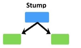
The third difference between random forest and Adaboost is, in the random forest, all the individual models are one fully grown decision tree. When we say ML model 1 or decision tree model 1, in the random forest that is a fully grown decision tree. In Adaboost, the trees are not fully grown. Rather the trees are just one root and two leaves. Specifically, they are called stumps in the language of Adaboost. Stumps are nothing but
one root node and two leaf nodes.
So, these are basic differences between how a bagging algorithm works and how a boosting algorithm works.
2. Understand Adaboost with data
Now we will take an example and try to understand how Adaboost works.
I consider a simple example here. You can see this data in 3 columns age, BMI, and gender.
| AGE | BMI | GENDER |
| 25 | 24 | F |
| 41 | 31 | F |
| 56 | 28 | M |
| 78 | 26 | F |
| 62 | 30 | M |
Let’s consider gender as the target column and the rest be the independent variable. Let say we try to fit a boosting algorithm or Adaboost on this data.
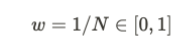
The very first thing it does is, it will assign a weight to all these records called initial weights. The initial weights would be a sum equal to 1.
| AGE | BMI | GENDER | INITIAL WEIGHTS |
| 25 | 24 | F | 1/5 |
| 41 | 31 | F | 1/5 |
| 56 | 28 | M | 1/5 |
| 78 | 26 | F | 1/5 |
| 62 | 30 | M | 1/5 |
Now, as I told you Adaboost is a sequential learning process, what will happen is the first model or
first-week learner or first base model will be fit on this data. So, as I told you here in Adaboost the weak learners are stumps that have one root and
two leaves.
This is one weak learner, the very first weak learner.
Now, you may ask how do we create this one stump?
The fundamental concept remains the same. Gini or index entropy whatever we take, the first two columns are the candidate columns for crating the root node. So, Gini index or entropic will be checked then a condition will be selected and then this stump will be created.
Once this stump is created, what will happen is this data will be tested for accuracy on this stump. There is a possibility that when the testing happens on this training data, some of this classification which this stump will do might go wrong.
So, let’s say this stump is created and then the testing happens on this data which produces the following results.
| AGE | BMI | GENDER | INITIAL WEIGHTS | PREDICTION |
| 25 | 24 | F | 1/5 | Correct |
| 41 | 31 | F | 1/5 | Correct |
| 56 | 28 | M | 1/5 | Wrong |
| 78 | 26 | F | 1/5 | Correct |
| 62 | 30 | M | 1/5 | Correct |
So, what happens in the next iteration is these initial weights are changed. This is very important for boosting techniques.
Initially, we started with giving similar weight to all the records which means all the records were equally important for the model. But what happens in the next iteration or next model is something that has been misclassified.
In this case, the third particular record has been misclassified by the previous model. So, what will happen is the weight for this record goes up and to normalize the entire weight, the weight for all other records comes down.
Now, in the next model the more importance is given to previously misclassified records or what happens in the next iteration or weak learner is this particular record will try to classify correctly with more weightage. So, the next learner will focus more on this particular record.
3. Final model
Here we are just talking about 5 records only. What if we have about 1 million records. There will be a good number of records that were misclassified by this weak learner and hence those records will be given higher weightage for the next learner or next ML model 2.
Similarly, this ML model 2 will misclassify some of the observations. That observation will again be given more weight and other observations’ weight will be coming down to normalize. Similarly, all the models will be created and whatever the misclassification happens in the previous model, the next model will try to classify it correctly. This is how in sequence one model takes the input from the previous model and tries to classify. This is adaptive boosting and that is why the name is adaptive boosting. Because it adapts to the previous model.
In the end, the final model is a model which is a combination of all these learnings and hence this technique is called boosting technique and this algorithm is called Adaboost.
The important thing to understand here is the initialization of weight and adjustment of weight based on misclassification, the internal fundamental concepts of creating a decision tree, creating stumps remain the same like gini entropy and all those things. But what is different here is these weights and it’s adjustments. This is how Adaboost works.
4. Mathematical explanation
There is a formula for the assignment of weights. The initial assignment of weights can be given
by,
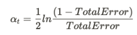
Here, N denotes the total number of data points. i.e. the number of records. The actual influence can be classified using
Where alpha denotes the influence of a particular stump in making the final decision. The total error is the total number of misclassified data. The sample weights can be updated using the following formula.
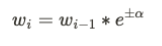
Here, the new sample weight is given by the multiplication of Euler’s number with the old sample weight.
alpha will be positive if the records are classified correctly else it will be negative.
5. Practical implementation with Python
First of all, we will load all the basic libraries.
import pandas as pd
import numpy as np
from sklearn.ensemble import AdaBoostClassifier
from sklearn.tree import DecisionTreeClassifier
from sklearn.datasets import load_breast_cancer
from sklearn.model_selection import train_test_split
from sklearn.metrics import confusion_matrix, accuracy_score
from sklearn.preprocessing import LabelEncoder
Here, I use the breast cancer dataset which can be obtained from sklearn.datasets. It is
also available in Kaggle.
breast_cancer = load_breast_cancer()
Let’sdeclare our independent variable and the target variable.
X = pd.DataFrame(breast_cancer.data, columns = breast_cancer.feature_names)
y = pd.Categorical.from_codes(breast_cancer.target, breast_cancer.target_names)
The target is to classify whether it is a benign or malignant cancer. So, let’s encode the target variable as 0 and 1. 0 for malignant, and 1 for benign.
encoder = LabelEncoder()
binary_encoded_y = pd.Series(encoder.fit_transform(y))
Now we split our dataset as train set and test set.
train_X, test_X, train_y, test_y = train_test_split(X, binary_encoded_y, random_state = 1)
we use the Adaboost classifier. Here, we use a decision tree for our model.
import pandas as pd
import numpy as np
from sklearn.ensemble import AdaBoostClassifier
from sklearn.tree import DecisionTreeClassifier
from sklearn.datasets import load_breast_cancer
from sklearn.model_selection import train_test_split
from sklearn.metrics import confusion_matrix, accuracy_score
from sklearn.preprocessing import LabelEncoder

breast_cancer = load_breast_cancer()

X = pd.DataFrame(breast_cancer.data, columns = breast_cancer.feature_names)
y = pd.Categorical.from_codes(breast_cancer.target, breast_cancer.target_names)

encoder = LabelEncoder()
binary_encoded_y = pd.Series(encoder.fit_transform(y))

train_X, test_X, train_y, test_y = train_test_split(X, binary_encoded_y, random_state = 1)

classifier = AdaBoostClassifier(DecisionTreeClassifier(max_depth=1), n_estimators=200)
classifier.fit(train_X, train_y)
print(classifier)
Our Adaboost is fitted now. We will predict the target variable in the test set now.
prediction = classifier.predict(test_X)
Let’s obtain the confusion matrix.
confusion_matrix(test_y, prediction)
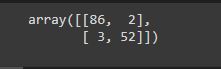
The main diagonal elements are well-classified data and secondary diagonal elements are misclassified data.
Let’s see the accuracy of classification now.
accuracy = accuracy_score(test_y, prediction)
print('AdaBoost Accuracy: ', accuracy)
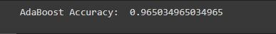
Our accuracy is 96.50%
It is quite a good accuracy.
6. Advantages and disadvantages
Coming to the advantages, Adaboost is less prone to overfitting as the input parameters are not jointly optimized. The accuracy of weak classifiers can be improved by using Adaboost. Nowadays, Adaboost is being used to classify text and images rather than binary classification problems.
The main disadvantage of Adaboost is that it needs a quality dataset. Noisy data and outliers have to be avoided before adopting an Adaboost algorithm.
7. References
Endnotes
By now, I am sure you will have an idea of Adaboost concepts. The actual fun in machine learning
begins once you start practicing. Take up problems, apply to code, and enjoy learning.
The media shown in this article are not owned by Analytics Vidhya and are used at the Author’s discretion


