This article was published as a part of the Data Science Blogathon
Introduction
You must have heard it by now, “Data is the new oil!”. In today’s digital world, there is an enormous amount of data floating around in various forms. There’s been a huge increase in image data, due to social media sites and apps. Deep learning is a field that specializes in working with image data. In this blog, I’ll build an image classifier using PyTorch API.
Wondering what are its applications?
You can find hundreds of examples around you. For example, when you open your Google Photos, you can find a collection called “Things”, under which there are categories like “Sky”, “Hiking”, “Temples”, “Cars” and so on. Google’s algorithm has classified your photos into one of these. Another main application is in the field of healthcare. Trained models can classify X-rays/scans as positive/negative for the disease.
Let’s start with binary classification, which is classifying an image into 2 categories, more like a YES/NO classification. Later, you could modify it and use it for multiclass classification also.
What’s our Data?
There are many datasets like MNIST, CIFAR10 upon which you can perform classification. For this blog, I have chosen a Kaggle dataset: Hot Dog – Not a hotdog. You can find the link here: https://www.kaggle.com/dansbecker/hot-dog-not-hot-dog
It basically has images that are either Hot dogs or not hot dogs.
You can visualize some samples like this from both classes
from PIL import Image
Image.open("../input/seefood/train/hot_dog/1053879.jpg")
Image.open("../input/seefood/train/not_hot_dog/102037.jpg")
Outputs:

It has two directories train and test. Our aim is to build a model, train it upon the training data and check its accuracy on the test dataset.
We’ll be using the Pytorch framework. It’s very popular due to its simple API for building and training models. As a first step let’s go ahead and import the main libraries and modules that’ll be required.
import pandas as pd
import matplotlib.pyplot as plt
import torch
import torchvision
import torch.nn as nn
import torch.optim as optim
import torch.nn.functional as F
from torchvision import transforms, utils, datasets
from torch.utils.data import Dataset, DataLoader
from torchvision import datasets
Processing the Dataset
You might often need to process the image data before passing it to the model. For example, if the sizes of all images are different (which often the case in large datasets), then your model will throw an error. So resize them, and you can consider rescaling the pixel values also. Apart from this, you can perform diverse transforms for data augmentation.
An elegant way to apply multiple transforms is using transform.compose() as shown below.
train_transform = transforms.Compose([transforms.Resize(255),transforms.RandomResizedCrop(224),
                                transforms.CenterCrop(224),
                                transforms.RandomHorizontalFlip(),
                                transforms.ColorJitter(),
                                transforms.ToTensor()])
test_transform = transforms.Compose([
                                transforms.Resize(255),
                                transforms.CenterCrop(224),
                                transforms.ToTensor()])
Pytorch provides inbuilt Dataset and DataLoader modules which we’ll use here. The Dataset stores the samples and their corresponding labels. While, the DataLoader wraps an iterable around the Dataset to enable easy access to the samples.
train_data = datasets.ImageFolder("train_data_directory", transform=train_transform)
test_data = datasets.ImageFolder("test_data_directory", transform=test_transform)
You can use the ImageFolder() function to pass the root directory containing samples and the transform you need to perform.
train_loader = torch.utils.data.DataLoader(train_data, batch_size=16,shuffle=True)
test_loader = torch.utils.data.DataLoader(test_data, batch_size=16)
The DataLoader() inputs the Dataset along with batch size. In the above code, I have called for a batch of 16 samples. You can use the shuffle argument to make sure the order of the data doesn’t affect the results.
You can check the shape of the inputs from your data loaders: (Batch size X No of channels X height X width)
Building the Model: Decrypting the layers
Here, we’ll write the architecture of the model we are going to use. We’ll define a class that derives from the PyTorch nn.Module. Inside the class, we’ll define the layers we want.
class Binary_Classifier(nn.Module):
    def __init__(self):
        super(CNN, self).__init__()
        self.conv1 = nn.Conv2d(in_channels=3, out_channels=10, kernel_size=3)
        self.conv2 = nn.Conv2d(10, 20, kernel_size=3)
        self.conv2_drop = nn.Dropout2d()
        self.fc1 = nn.Linear(720, 1024)
        self.fc2 = nn.Linear(1024, 2)

    def forward(self, x):
        x = F.relu(F.max_pool2d(self.conv1(x), 2))
        x = F.relu(F.max_pool2d(self.conv2_drop(self.conv2(x)), 2))
        x = x.view(x.shape[0],-1)
        x = F.relu(self.fc1(x))
        x = F.dropout(x, training=self.training)
        x = self.fc2(x)
        return x
The model class definition should always have __init__() method. In this, we will initialize the blocks/layers and other parameters.
Talking about the neural network layers, there are 3 main types in image classification: convolutional, max pooling, and dropout .
Convolution layers
Convolutional layers will extract features from the input image and generate feature maps/activations. You can decide how many activations you want using the filters argument. Basically, when you apply convolution upon an image, the kernel will pass over the entire image in small parts, and it will give an activation. It is demonstrated in the below image.
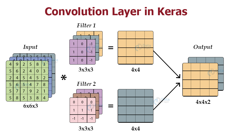
source: Image
Pooling Layers
When we use conv2d layers, we end up with a lot of feature maps that occupy high computational space. In order to decrease the computational time and space required, you can use Max pooling or average pooling. For each patch/group of the map, only the maximum is chosen to form the output. The below image clearly demonstrates the work.
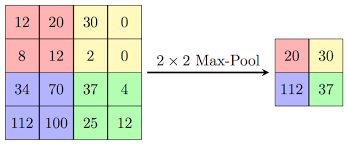
source : Image
Dropout Layers
You can guess its function from the name itself! It drops out like 10-20% of the data.
Wonder why?
Overfitting is a common problem when you are training over the same data for many iterations/epochs. By dropping out a randomly chosen 10% of data, the model will be able to generalize more to new data.
This concludes with a brief description of the layers we have used in our code. Note that the final layer has output as 2, as it is binary classification.
Hence, our model is ready!
Training the Model
Finally comes the training part. Here you need to decide two crucial things: Loss function and optimizer. There are various choices like SGD, Adam, etc.. for the optimizer. I have used Cross-Entropy loss, which is a popular choice in the case of classification problems. You should also set a learning rate, which decides how fast your model learns.
model=Binary_Classifier()
criterion = nn.CrossEntropyLoss()
optimizer = torch.optim.Adam(model.parameters(),lr = learning_rate)
Initialize the model from the class definition. Next, you have to decide how many epochs to train. You can loop over the batches of data from the train loader, and pass the image to the forward function of the model we defined earlier.
train_losses = []
for epoch in range(1, num_epochs=15):
    train_loss = 0.0
    model.train()
    for data, target in train_loader:

        optimizer.zero_grad()
         forward-pass
        output = model(data)
        loss = criterion(output, target)
        #backward-pass
        loss.backward()
        # Update the parameters
        optimizer.step()
        # Update the Training loss
        train_loss += loss.item() * data.size(0)
After the forward pass, the prediction is returned. We pass the prediction and the label to the loss criterion. It computes and returns the cross-entropy loss. Then, we compute the backward pass. That is, we compute the gradient of the loss with respect to the weights. After this, the weights are updated. Do not forget to do zero_grad() at the end or at the beginning. It clears the previously calculated gradients.
Yay! we have successfully trained a Binary Classifier. You can test it and tune hyperparameters to achieve better results.
Thanks for reading! You can connect with me at: [email protected]
The media shown in this article are not owned by Analytics Vidhya and are used at the Author’s discretion.


You copied the CNN model form Uni of Toronto without giving credit. In this process you forgot to rename your super init from CNN to Binary_Classifier