This article was published as a part of the Data Science Blogathon
Introduction
VGG- Network is a convolutional neural network model proposed by K. Simonyan and A. Zisserman in the paper “Very Deep Convolutional Networks for Large-Scale Image Recognition” [1]. This architecture achieved top-5 test accuracy of 92.7% in ImageNet, which has over 14 million images belonging to 1000 classes.
It is one of the famous architectures in the deep learning field. Replacing large kernel-sized filters with 11 and 5 in the first and second layer respectively showed the improvement over AlexNet architecture, with multiple 3×3 kernel-sized filters one after another. It was trained for weeks and was using NVIDIA Titan Black GPU’s.
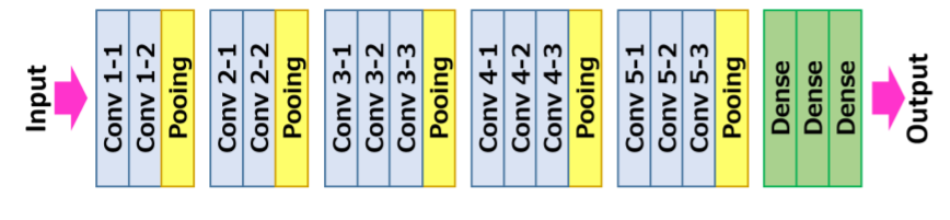
VGG16 Architecture
The input to the convolution neural network is a fixed-size 224 × 224 RGB image. The only preprocessing it does is subtracting the mean RGB values, which are computed on the training dataset, from each pixel.
Then the image is running through a stack of convolutional (Conv.) layers, where there are filters with a very small receptive field that is 3 × 3, which is the smallest size to capture the notion of left/right, up/down, and center part.
In one of the configurations, it also utilizes 1 × 1 convolution filters, which can be observed as a linear transformation of the input channels followed by non-linearity. The convolutional strides are fixed to 1 pixel; the spatial padding of convolutional layer input is such that the spatial resolution is maintained after convolution, that is the padding is 1 pixel for 3 × 3 Conv. layers.
Then the Spatial pooling is carried out by five max-pooling layers, 16 which follow some of the Conv. layers but not all the Conv. layers are followed by max-pooling. This Max-pooling is performed over a 2 × 2-pixel window, with stride 2.
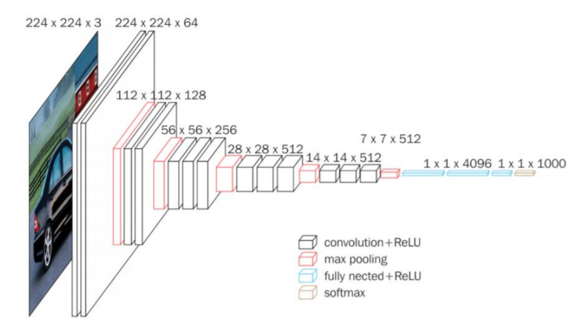
The architecture contains a stack of convolutional layers which have a different depth in different architectures which are followed by three Fully-Connected (FC) layers: the first two FC have 4096 channels each and the third FC performs 1000-way classification and thus contains 1000 channels that is one for each class.
The final layer is the soft-max layer. The configuration of the fully connected layers is similar in all networks.
All of the hidden layers are equipped with rectification (ReLU) non-linearity. Also, here one of the networks contains Local Response Normalization (LRN), such normalization does not improve the performance on the trained dataset, but usage of that leads to increased memory consumption and computation time.
Architecture Summary:
• Input to the model is a fixed size 224×224224×224 RGB image
• Pre-processing is subtracting the training set RGB value mean from each pixel
• Convolutional layers 17
– Stride fixed to 1 pixel
– padding is 1 pixel for 3×33×3
• Spatial pooling layers
– This layer doesn’t count to the depth of the network by convention
– Spatial pooling is done using max-pooling layers
– window size is 2×22×2
– Stride fixed to 2
– Convnets used 5 max-pooling layers
• Fully-connected layers:
• 1st: 4096 (ReLU).
▪ 2nd: 4096 (ReLU).
▪ 3rd: 1000 (Softmax).
Architecture Configuration
The below figure contains the Convolution Neural Network configuration of the VGG net with the
following layers:
• VGG-11
• VGG-11 (LRN)
• VGG-13
• VGG-16 (Conv1)
• VGG-16
• VGG-19
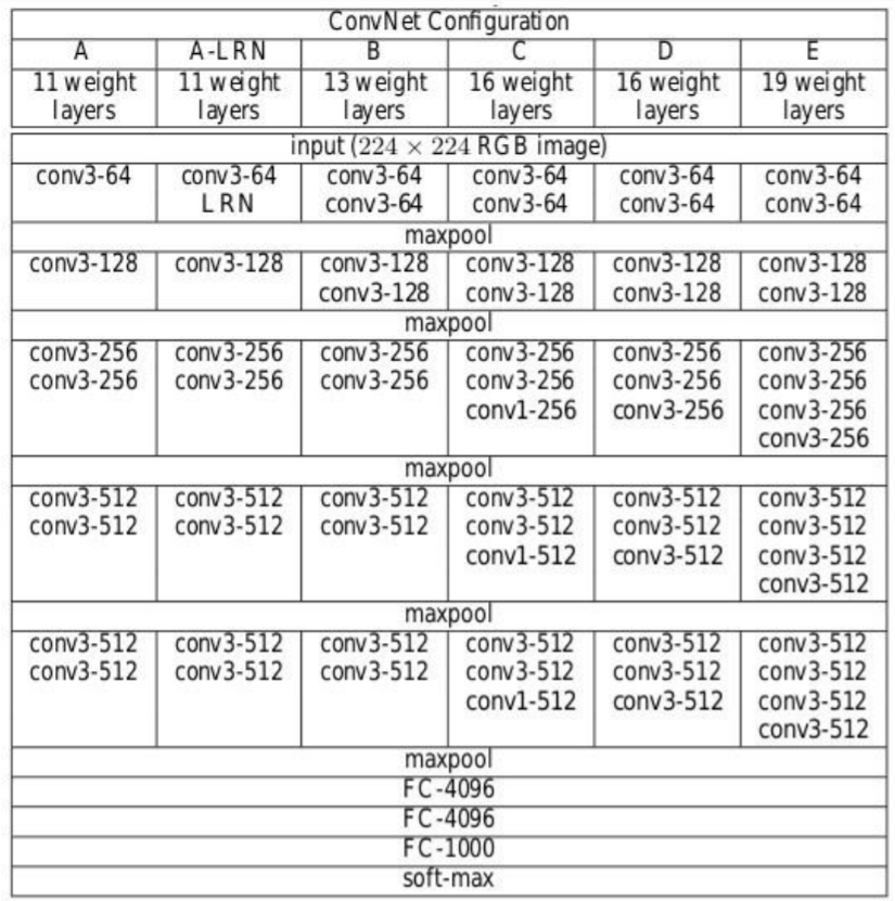
Source: ‘Very Deep Convolutional Networks For Large-Scale Image Recognition”
The convolutional Neural Network configurations are mentioned above one per column.
In the following, the networks are referred by their names (A–E). All configurations follow the traditional design and differ only in the depth: from 11 weight layers in network A that is 8 Conv. and 3 FC layers to 19 weight layers in network E that is 16 Conv. and 3 FC layers. The width of each Conv. layer is the number of channels is rather small, which is starting from 64 in the first layer and then goes on increasing by a factor of 2 after each max-pooling layer until it reaches 512.
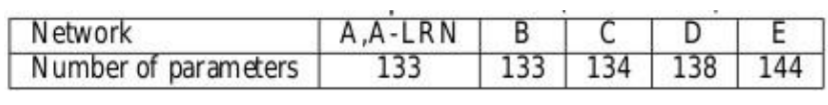
The number of parameters for each configuration is described below. Although it has a large depth, the number of weights in the networks is not greater than the number of weights in a shallower net with larger Conv. layer widths and receptive fields
Training
• Loss function is multinomial logistic regression
• Learning algorithm is mini-batch stochastic gradient descent (SGD) based on back-propagation with momentum
· Batch size was 256
· Momentum was 0.9
• Regularization
· L2 Weight decay (penalty multiplier was 0.0005)
· Dropout for first two fully connected layers is set to 0.5
• Learning rate
· Initial: 0.01
· When validation set accuracy stopped improving it is decreased to 10.
• Though it has a greater number of parameters and also depth compared to Alexnet, the CNN’s required less epochs for loss function to converge due to
· Small convolutional kernels and more regularization by large depth.
· Pre-initialization of certain layers.
• Training image size
· S is the smallest side of the isotopically-rescaled image
· Two approaches for setting S
▪ Fix S, known as single scale training
▪ Here S = 256 and S = 384
▪ Vary S, known as multi-scale training
▪ S from [Smin, Smax] where Smin = 256, Smax = 512
– Then 224×224224×224
the image was randomly cropped from rescaled image per SGD iteration.
Key Features
• VGG16 has a total of 16 layers that has some weights.
• Only Convolution and pooling layers are used.
• Always uses a 3 x 3 Kernel for convolution. 20
• 2×2 size of the max pool.
• 138 million parameters.
• Trained on ImageNet data.
• It has an accuracy of 92.7%.
• Another version that is VGG 19, has a total of 19 layers with weights.
• It is a very good Deep learning architecture for benchmarking on any particular task.
• The pre-trained networks for VGG is made open-source, so it can be commonly used out of the box for various types of applications.
Let’s Implement VGG Net
First Let’s create the filter mapping for each version of the VGG net. Refer to the above configuration image to know about the number of filters. That is create a dictionary for the version with a key named VGG11, VGG13, VGG16, VGG19 and create a list according to the number of filters in each version respectively. Here “M” in the list is known as Maxpool operation.
import torch
import torch.nn as nn
VGG_types = {
"VGG11": [64, "M", 128, "M", 256, 256, "M", 512, 512, "M", 512, 512, "M"],
"VGG13": [64, 64, "M", 128, 128, "M", 256, 256, "M", 512, 512, "M", 512, 512, "M"],
"VGG16": [64,64,"M",128,128,"M",256,256,256,"M",512,512,512,"M",512,512,512,"M",],
"VGG19": [64,64,"M",128,128,"M",256,256,256,256,"M",512,512,512,512,
          "M",512,512,512,512,"M",],}
Create a global variable to mention the version of the architecture. Then create a class called VGG_net with inputs as in_channels and num_classes, It takes inputs like a number of Image channels and the Number of output classes.
Initialize the Sequential layers, that is in the sequence, Linear layer–>ReLU–>Dropout.
Then create a function called create_conv_layers which takes VGGnet architecture configuration as input that is the list that we created above for different versions. When it comes across the letter “M” from the above list, it performs the MaxPool2d operation.
VGGType = "VGG16"
class VGGnet(nn.Module):
    def __init__(self, in_channels=3, num_classes=1000):
        super(VGGnet, self).__init__()
        self.in_channels = in_channels
        self.conv_layers = self.create_conv_layers(VGG_types[VGGType])
self.fcs = nn.Sequential(
nn.Linear(512 * 7 * 7, 4096),
nn.ReLU(),
nn.Dropout(p=0.5),
nn.Linear(4096, 4096),
nn.ReLU(),
nn.Dropout(p=0.5),
nn.Linear(4096, num_classes),
)

def forward(self, x):
x = self.conv_layers(x)
x = x.reshape(x.shape[0], -1)
x = self.fcs(x)
return x

def create_conv_layers(self, architecture):
layers = []
in_channels = self.in_channels

for x in architecture:
if type(x) == int:
out_channels = x

layers += [
nn.Conv2d(
in_channels=in_channels,
out_channels=out_channels,
kernel_size=(3, 3),
stride=(1, 1),
padding=(1, 1),
),
nn.BatchNorm2d(x),
nn.ReLU(),
]
in_channels = x
elif x == "M":
layers += [nn.MaxPool2d(kernel_size=(2, 2), stride=(2, 2))]

return nn.Sequential(*layers)
Once this is done write a small test code to check whether our implementation is working well.
In the below test code the number of classes given is 500.
if __name__ == "__main__":
    device = "cuda" if torch.cuda.is_available() else "cpu"
    model = VGGnet(in_channels=3, num_classes=500).to(device)
    # print(model)
    x = torch.randn(1, 3, 224, 224).to(device)
    print(model(x).shape)
The output should be like this:
If you want to see the network architecture you can uncomment the print(model) statement from the above code. Also can try with different versions by changing the VGG versions in the variable VGGType.
The entire code can be accessed here:
https://github.com/BakingBrains/Deep_Learning_models_implementation_from-scratch_using_pytorch_/blob/main/VGG.py
[1]. K. Simonyan and A. Zisserman: Very Deep Convolutional Networks for Large-Scale Image Recognition, April 2015, DOI: https://arxiv.org/pdf/1409.1556.pdf
Thank You
The media shown in this article are not owned by Analytics Vidhya and are used at the Author’s discretion.
I thrive on the thrill of the challenge, tackling complex problems and crafting innovative AI solutions that make a difference. Whether it's optimizing or building sustainable AI ecosystems, I believe in harnessing the power of AI for the greater good. Let's brainstorm, collaborate, and change the world, one byte at a time.


