Classification Problem: Relation between Sensitivity, Specificity and Accuracy
This article was published as a part of the Data Science Blogathon
Introduction
The model performance in a classification problem is assessed through a confusion matrix. The elements of the confusion matrix are utilized to find three important parameters named accuracy, sensitivity, and specificity. The prediction of classes for the data in a classification problem is based on finding the optimum boundary between classes. Based on the values of accuracy, sensitivity, and specificity one can find the optimum boundary. This article explains the relation between sensitivity, specificity and accuracy and how together they can help to determine the optimum boundary.
Confusion Matrix
In any machine learning model, we usually focus on accuracy. But if you are dealing with a classification problem, you also need to worry about the percentage of correct classification and misclassification. So we need a mechanism that not only provides accuracy but also helps in estimating correct classification and misclassification. The confusion matrix serves this purpose. It is an NxN matrix which helps to evaluate the performance of machine learning model for classification problem. Figure 1 presents the confusion matrix for the binary class classification problem.
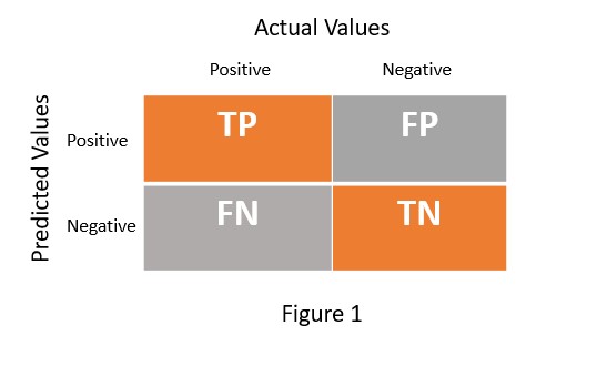
TP = True Positive
TN = True Negative
FP = False Positive
FN = False Negative
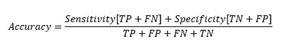
From the confusion matrix Accuracy, Sensitivity and Specificity is evaluated using the following equations
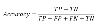
Accuracy Formula

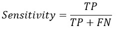
Sensitivity Formula

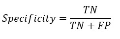
Specificity Formula
Example – Calculate Confusion Matrix
We will take a simple binary class classification problem to calculate the confusion matrix and evaluate accuracy, sensitivity, and specificity. Diabetes in the patient is predicted based on the data of blood sugar level.
Dataset – Download diabetes_data.csv. This dataset is the simplified version of diabetes data available at Kaggle.
We will build the model and calculate the confusion matrix using a step-by-step approach.
Step 1- Import Data
import pandas as pd
import numpy as np
dib = pd.read_csv('diabetes_data.csv') # Import data in dataframe named dibdib.shape # Understand shape of the dataframe(768, 2) #The dataset has 768 rows and 2 columnsdib.head() # Look at few rows| Blood Sugar Level | Diabetes | |
|---|---|---|
| 0 | 148 | Yes |
| 1 | 85 | No |
| 2 | 183 | Yes |
| 3 | 89 | No |
| 4 | 137 | Yes |
The dataset has two columns. Diabetes is dependent or response variable. And Blood Sugar Level is an independent variable or feature variable to predict diabetes.
Step 2: Feature Engineering
Certain modifications in the dataset will be done to make it suitable for modeling
dib['Diabetes'] = dib['Diabetes'].map({'Yes': 1, 'No': 0}) # Converting Yes to 1 and No to 0X = dib['Blood Sugar Level'] # Putting feature variable to X
y = dib['Diabetes'] # Putting response variable to yStep 3: Split data into train and test
The dataframe dib will be split into train and test. The training dataset will be used to build the model
from sklearn.model_selection import train_test_split
X_train, X_test, y_train, y_test = train_test_split(X, y, train_size=0.7, test_size=0.3, random_state=100)
Step 4: Build a binary classification model
import statsmodels.api as sm
X_train_sm = sm.add_constant(X_train)
logm2 = sm.GLM(y_train,X_train_sm, family = sm.families.Binomial())
res = logm2.fit()
res.summary()
y_train_pred = res.predict(X_train_sm) #Predict blood sugar level
Step 5: Predict Diabetes
Based on training data we will create a new dataframe named dib_train which will include original and predicted diabetes
data = {'Blood Sugar Level':X_train, 'Diabetes':y_train, 'y_train_pred':y_train_pred}
dib_train = pd.DataFrame(data)
Create predicted diabetes based on a 0.5 cut-off probability
dib_train['Diabetes_predicted'] = dib_train.y_train_pred.map(lambda x: 1 if x > 0.5 else 0)
dib_train.head()| Blood Sugar Level | Diabetes | y_train_pred | Diabetes_predicted | |
|---|---|---|---|---|
| 155 | 152 | 1 | 0.612023 | 1 |
| 150 | 136 | 0 | 0.455384 | 0 |
| 78 | 131 | 1 | 0.406777 | 0 |
| 9 | 125 | 1 | 0.350842 | 0 |
| 142 | 108 | 0 | 0.215890 | 0 |
As can be seen from the table, there is a certain wrong prediction or misclassification. The correct classification and misclassification are determined by the confusion matrix. The percentage of misclassification is dependent upon the choice of cut-off. We will evaluate the optimum cut-off in the next few steps.
Step 6: Confusion Matrix and Accuracy
Now let’s evaluate the confusion matrix
# Confusion matrix
from sklearn import metrics
confusion = metrics.confusion_matrix(dib_train.Diabetes, dib_train.Diabetes_predicted)
print(confusion)
[[309  41]
 [ 96  91]]
# Let's check the overall accuracy.
print(metrics.accuracy_score(dib_train.Diabetes, dib_train.Diabetes_predicted))
0.74487895716946
Step 7: Variation with Cut-Off
So far, we have calculated the confusion matrix and accuracy with cut-off=0.5. This assumes that the data is divided exactly at 0.5 probability. Now let’s vary the probability from 0.1 to 0.9.
# Let's calculate Sensitivity, Specificity and accuracy with different probability cutoffs

numbers = [float(x)/10 for x in range(10)]

for i in numbers:
    dib_train[i]= dib_train.y_train_pred.map(lambda x: 1 if x > i else 0)
dib_train.head()| Blood Sugar Level | Diabetes | y_train_pred | Diabetes_predicted | 0.0 | 0.1 | 0.2 | 0.3 | 0.4 | 0.5 | 0.6 | 0.7 | 0.8 | 0.9 | |
|---|---|---|---|---|---|---|---|---|---|---|---|---|---|---|
| 155 | 152 | 1 | 0.612023 | 1 | 1 | 1 | 1 | 1 | 1 | 1 | 1 | 0 | 0 | 0 |
| 150 | 136 | 0 | 0.455384 | 0 | 1 | 1 | 1 | 1 | 1 | 0 | 0 | 0 | 0 | 0 |
| 78 | 131 | 1 | 0.406777 | 0 | 1 | 1 | 1 | 1 | 1 | 0 | 0 | 0 | 0 | 0 |
| 9 | 125 | 1 | 0.350842 | 0 | 1 | 1 | 1 | 1 | 0 | 0 | 0 | 0 | 0 | 0 |
| 142 | 108 | 0 | 0.215890 | 0 | 1 | 1 | 1 | 0 | 0 | 0 | 0 | 0 | 0 | 0 |
 from sklearn.metrics import confusion_matrix
# TP = confusion[1,1] # true positive
# TN = confusion[0,0] # true negatives
# FP = confusion[0,1] # false positives
# FN = confusion[1,0] # false negatives
num = [0.0,0.1,0.2,0.3,0.4,0.5,0.6,0.7,0.8,0.9]
for i in num:
    cm1 = metrics.confusion_matrix(dib_train.Diabetes, dib_train[i])
    total1=sum(sum(cm1))
    Accuracy = (cm1[0,0]+cm1[1,1])/total1
    Specificity = cm1[0,0]/(cm1[0,0]+cm1[0,1])
    Sensitivity = cm1[1,1]/(cm1[1,0]+cm1[1,1])
    cutoff_df.loc[i] =[ i ,Accuracy,Sensitivity,Specificity]
# # Let's plot accuracy sensitivity and specificity for various probabilities.
import matplotlib.pyplot as plt
cutoff_df = pd.DataFrame( columns = ['Probability','Accuracy','Sensitivity','Specificity'])
plt.show()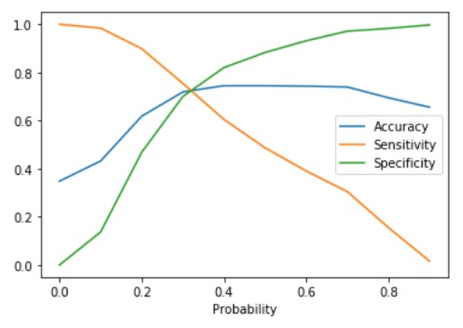
The plot between sensitivity, specificity, and accuracy shows their variation with various values of cut-off. Also can be seen from the plot the sensitivity and specificity are inversely proportional. The point where the sensitivity and specificity curves cross each other gives the optimum cut-off value. This value is 0.32 for the above plot. Let us calculate the value of Sensitivity, Specificity, and accuracy at the optimum point.
dib_train['Diabetes_predicted'] = dib_train.y_train_pred.map(lambda x: 1 if x > 0.32 else 0)
# Let's check the overall accuracy.
print(metrics.accuracy_score(dib_train.Diabetes, dib_train.Diabetes_predicted))
0.7281191806331471
# Confusion matrix
confusion = metrics.confusion_matrix(dib_train.Diabetes, dib_train.Diabetes_predicted)
print(confusion)
[[253 97]TP = confusion[1,1] # true positive
TN = confusion[0,0] # true negatives
FP = confusion[0,1] # false positives
FN = confusion[1,0] # false negatives
# Let's see the sensitivity of our logistic regression model

TP / float(TP+FN)

0.7379679144385026
# Let us calculate specificity
TN / float(TN+FP)0.7228571428571429
We can see that the value of Sensitivity and Specificity are close to each other for optimum
cut-off point. One interesting observation from the above analysis is that accuracy is also
same at the point where sensitivity and specificity cross each other.
Why accuracy is also the same at the point where sensitivity and specificity cross each other is explained in the next section.
Accuracy at Sensitivity and Specificity Crossing Point

Replacing TP and TN from Sensitivity and Specificity equation-
At cut-off point-
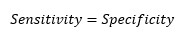
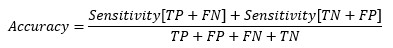
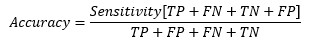

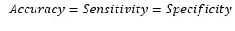
So, at the cut-off point where sensitivity and specificity are equal, the accuracy is also the same.
Conclusion
This article presented the relation between Sensitivity ,Specificity and Accuracyin a classification problem. The sensitivity and Specificity are inversely proportional. And their plot with respect to cut-off points crosses each other. The cross point provides the optimum cutoff to create boundaries between classes. At the optimum cut-off or crossing point, the sensitivity and specificity are equal. And through mathematical derivation, we also saw that at the optimum cut-off point the accuracy is also equal to Sensitivity and Specificity.
Frequently Asked Questions
A. The formula for specificity is as follows:
Specificity = True Negative / (True Negative + False Positive)
A. he formula for sensitivity, also known as the true positive rate or recall, is as follows:
Sensitivity = True Positive / (True Positive + False Negative)
Code
The code for the article can be found https://github.com/mokhanna/Diabetes-Prediction
About Me
My name is Mohit Khanna. I am working in Software Industry. Data Science and Machine Learning is my recent interest area.
The media shown in this article are not owned by Analytics Vidhya and are used at the Author’s discretion.


