Complete Guide to Prevent Overfitting in Neural Networks (Part-2)
This article was published as a part of the Data Science Blogathon
Introduction
This is the final part of two-part Blog Series on Regularization Techniques for Neural Networks.
In the first part of the blog series, we discuss the basic concepts related to Underfitting and Overfitting and learn the following three methods to prevent overfitting in neural networks:
- Reduce the Model Complexity
- Data Augmentation
- Weight Regularization
For part-1 of this series, refer to the link.
So, in continuation of the previous article, In this article we will cover the following techniques to prevent Overfitting in neural networks:
- Dropout
- Early Stopping
- Weight Decay
Important Note
After the completion of each of the techniques, there is some practice (Test your Knowledge) questions given that you have to solve and give the answer in the comment box so that you can check your understanding of a particular technique.
Dropout
It is another regularization technique that prevents neural networks from overfitting. Regularization methods like L1 and L2 reduce overfitting by modifying the cost function but on the contrary, the Dropout technique modifies the network itself to prevent the network from overfitting.
Working Principle behind this Technique
It randomly drops some neurons except for the output layer from the neural network during training in each iteration or we can assign a probability p to all the neurons in a network so that they are temporarily ignored from calculations.
where p is known as the Dropout Rate and is usually instantiated to 0.5.
Then, as each iteration is going on, the neurons in each layer with the highest probability get dropped. This results in creating a smaller network with each pass on the training dataset(epoch). Since in each iteration, a random input value can be eliminated, the network tries to balance the risk and not to favor any of the features and reduces bias and noise.
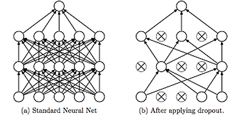
Image Source: Google Images
Sometimes, this technique is also known as the Ensemble Technique for Neural Networks as when we drop different sets of neurons, it’s equivalent to training different neural networks. So, in this technique, the different networks will overfit in different ways, so the net effect of dropout will be to reduce overfitting.
This technique to prevent overfitting has proven to reduce overfitting to a variety of problem statements that include,
- Image classification,
- Image segmentation,
- Word embedding,
- Semantic matching etcetera, etc.
Test Your Knowledge
Question-1: Do you think there is any connection between the dropout rate and regularization? For this question, you have to consider the dropout rate as the probability of keeping a neuron active.
Question-2: Suppose we have a 5-layer neural network that takes 4 hours to coach on a GPU with 4GB VRAM. At test time, it takes 3 seconds for a single datum.
Now we modify the architecture such we add dropout after the 2nd and 4th layer with rates of 0.3 and 0.5 respectively. Then, comment on the new testing time for this new architecture. Is it Less than 3 secs, Exactly 3 secs, or Greater than 3 secs?
Early Stopping
Early stopping is a form of regularization technique that applies when we training a model with an iterative method, such as Gradient Descent. Since all the neural networks learn exclusively with the help of optimization algorithms such as gradient descent, therefore early stopping is a technique applicable to all the problems. This technique prevents overfitting by updates the model so as to make it better fit the training data with each iteration.
As we know that too much training happening in the neural networks results in network overfitting on the training data.
Up to a certain point, the model performance on the test set improves. Before that point, however, improving the model’s fit to the training data leads to increased generalization error. This technique of regularization provides us a guide on how many iterations can be run before the model begins to overfit.
This technique is shown in the below diagram.
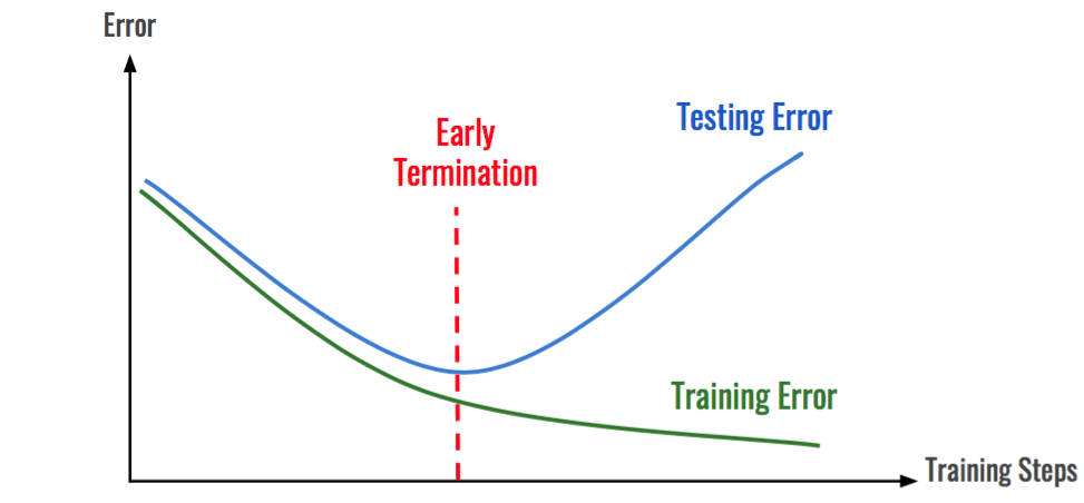
Image Source: Google Images
As we can see, after some iterations, the test error has started to increase while the training error is still decreasing. Hence the model is overfitting. So to resolve this problem, we stop the model at the point when this starts to happen.
The network parameters at the point of early termination are considered the best fit for the model. To decrease the test error beyond the point of early termination, the following ways can be used:
- Decreasing the learning rate. Use a learning rate scheduler algorithm would be recommended.
- Use a different Optimization Algorithm.
- Use weight regularization techniques like L1 or L2 regularization.
Test Your Knowledge
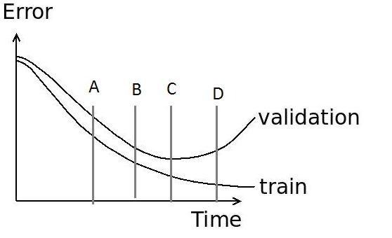
In the Image Recognition Task, while training a neural network we plot the graph of training error and validation error for debugging the network. Then, according to you what is the best place among A, B, C, and D within the graph for early stopping?
Weight Decay
In my part-1 article, I described that the data augmentation technique helps deep learning models to generalize well. That was on the data side of things. What about the model side of things?
So, the question comes to mind:
What can we do while training our models, so that our model is generalized well?
Parameters of a model
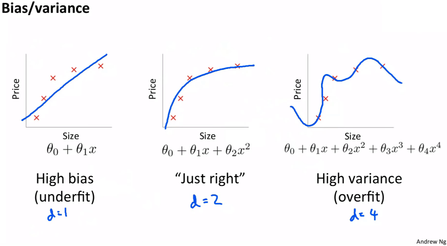
Image Source: Google Images
In the image shown above, we have a set of data points and by using the straight line, we cannot fit them well. Hence, we try to fit a 2nd-degree polynomial to do so but we notice that as the degree of the polynomial increases beyond a certain point, then our model becomes too complex and starts to overfit.
So, from the above diagram, we can understand that to prevent overfitting, we shouldn’t allow our models to get too complex. Unfortunately, this has led to a misconception in deep learning that we shouldn’t use a lot of parameters (in order to keep our models from getting overly complex).
How Weight Decay was Originated?
First of all, we have to understand that the real-world data is not going to be as simple as the one shown in the above picture. Real-world data is very complex and to solve complex problems, we required complex solutions.
Having few learnable parameters is only a single way to prevent our model from overfitting. But it is actually a very limiting strategy.
And one thing to note that is as there are more parameters in the networks, it results in more interactions between various parts of our neural network. And more interactions mean more non-linearities. These non-linearities help us solve complex problems.
However, our aim is to maintain these interactions or don’t want these interactions to get out of hand.
Hence, What if we penalize complexity?
After penalizing the complexity, we will still use that many parameters, but our aim is to prevent our model from getting too complex. This is exactly the idea of the weight decay technique to prevent neural networks from overfitting.
This thing called a Weight Decay
To penalize our model, one technique to penalize its complexity would be to add all our parameters (weights) to our loss function. Well, that won’t quite work because some parameters are positive and some are negative. So, we try to add the squares of all the parameters to our loss function. However, the problem with that thing is that it might result in our loss getting so huge that the best model would be to set all the parameters to 0.
To come out from the above problem, we multiply the overall sum of squares with another smaller number, which is called weight decay or wd.
Therefore, our new loss function becomes:
Loss = MSE(y_hat, y) + wd * sum(w2)
where,
y_hat and y are the predicted and actual values respectively.
MSE stands for Mean Squared Error.
Now, using gradient descent, we update our weights according to the given below formula:
w(t) = w(t-1) – lr * dLoss / dw
Now after penalizing, our loss function has two components in it, therefore the derivative of the 2nd term w.r.t w would be:
d(wd * w2) / dw = 2 * wd * w (similar to d(x2)/dx = 2x)
Now on, we will apply this formula which not only subtracts the learning rate * gradient from the weights but also 2 * wd * w. We are subtracting constant times the weight from the original weight. This is why it is known as weight decay.
Test Your Knowledge
Now, after learning the weight decay technique, it might seem that the weight decay technique is the same as the L2 regularization. Do you think this is true? Why or Why not?
This ends our Blog series on Regularization Techniques in Neural Networks!
End Notes
Thanks for reading!
If you liked this and want to know more, go visit my other articles on Data Science and Machine Learning by clicking on the Link
Please feel free to contact me on Linkedin, Email.
Something not mentioned or want to share your thoughts? Feel free to comment below And I’ll get back to you.
Frequently Asked Questions
A. Overfitting in neural networks occurs when a model learns to perform exceptionally well on the training data but fails to generalize to new, unseen data. It memorizes noise and specific examples, leading to poor performance on real-world tasks. This happens when the network is too complex or trained for too long, capturing noise instead of genuine patterns, resulting in decreased performance on new data.
A. You can detect neural network overfitting through various methods:
1. Validation Loss: If training loss drops but validation loss starts rising, overfitting is likely.
2. Learning Curve: Plotting training and validation performance over epochs can show divergence.
3. Validation Accuracy: If training accuracy is high but validation accuracy is low, overfitting might be present.
4. Regularization: Lack of regularization can contribute to overfitting.
5. Data Split: Separate datasets for training, validation, and testing help identify overfitting.
About the Author
Chirag Goyal
Currently, I am pursuing my Bachelor of Technology (B.Tech) in Computer Science and Engineering from the Indian Institute of Technology Jodhpur(IITJ). I am very enthusiastic about Machine learning, Deep Learning, and Artificial Intelligence.
The media shown in this article are not owned by Analytics Vidhya and are used at the Author’s discretion.
I am currently pursuing my Bachelor of Technology (B.Tech) in Computer Science and Engineering from the Indian Institute of Technology Jodhpur(IITJ). I am very enthusiastic about Machine learning, Deep Learning, and Artificial Intelligence. Feel free to connect with me on Linkedin.


