This article was published as a part of the Data Science Blogathon
“Time flies over us, but leave its shadow behind”
a beautiful quote by Nathaniel Hawthorne just says the truth about existence.
Whatever we do, we did or will do, one of the biggest determinants for all those actions is time. This clearly gets reflected in data available around us as well. Every single day billions of sensors(in all the domains of technology) are taking their readings and storing all that data in such a way that tracks the timestamps of their activity. We observe regularities and irregularities both with the comparison of those values with their past behaviour. ‘past’ shows behavior with correspondence to time already passed.
Unfolding some common words with respect to time:
1. Temporal: relating to or denoting time or tense. for example, there is a temporal shift in temperature. Now here, temporal shift corresponds to the change in values (shift in values) with respect to passing time.
2. Timestamp: An exact instance in time. Timestamp signifies when exactly something occurred/took place. Let’s see some examples, 2005-10-30 T 10:45 UTC is one of the representations of a timestamp. This one gives the information that the event took place on 30th October(10) 2005 at time 10:45 UTC (Coordinate Universal time).
From machine learning’s perspective, we often see data as either numerical or categorical and either image or textual and etc. The first thought that comes to our mind while observing numerical data values is to use regression to find out features that are relative to the label and helps us get a machine learning model for predictions. Well, after today you will be thinking more before reaching any conclusion because values can be relative to themselves on a temporal basis. There might be some behaviours in your numerical data which can help you get the future values just by learning the representation of past values with the future values.
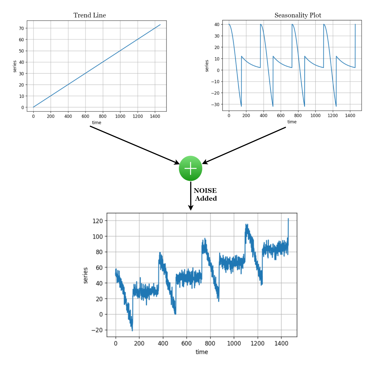
Let’s understand this with some synthetic time series data (don’t worry about the maths of how we created it, just focus on the values and their noticeable behaviour with time).
1. Generating Synthetic Time-series Data
To avoid redundancy with every time we plot the time series data, let’s make a helper function.
def plot_series(time, series, format="-", start = 0, end=None):
    plt.plot(time[start:end], series[start:end], format)
    plt.xlabel("time")
    plt.ylabel("series")
    plt.grid(True)
Functions to generate certain properties of time series: (Trend and Seasonality)
1. Trend: The linear regression line that you often see (linear line with certain slope and intercept) is what informs us about the trend in the data. How much did the values increase OR decrease during a certain time period.
2. Seasonality: Repetition of certain behaviours over a fixed time period is what we call seasonality. Let’s say for example that at the beginning of every month, a company earns 10% more than the rest of the month, we can say that a 10% revenue increment for the company is monthly seasonal. The behaviour repeats itself every month.
For the synthetic time series, we will merge both these properties of time series as function calls with a pre-determined intercept (AKA baseline).
def trend(time, slope= 0):
    return slope*time
def seasonal_pattern(season_time):
    return np.where(season_time<0.4,
                  np.cos(season_time*2*np.pi),
                  1/np.exp(3*season_time))
def seasonality(time, period, amplitude=1, phase=0):
    season_time = ((time+phase) % period)/period
    return amplitude*seasonal_pattern(season_time)
def noise(time, noise_level=1, seed=None):
    rnd = np.random.RandomState(seed)
    return rnd.randn(len(time))*noise_level
time = np.arange(4*365+1, dtype="float32")
baseline = 10
series = trend(time, 0.1)
baseline = 10
amplitude = 40
slope = 0.05
noise_level = 5
After we merge all that has been discussed this is what it would look like:
series = baseline + trend(time, slope) + seasonality(time, period=365, amplitude=amplitude)
# update the series with Noise
series+=noise(time, noise_level, seed=42)
Here is how you can visualize your time series using the helper function that we defined earlier.
plot_series(range(len(series)), series)
2. Preparing the Dataset
1. Dividing the series into the Training and Testing dataset.
NOTE: Here, you don’t shuffle the data before training, because their sequence is what our features will be, so shuffling would completely destroy the temporal patterns hidden in the data. We can only shuffle once we create batches of data that have their sequence intact inside, and their next immediate value after the batch ends would be their label to predict.
To make this more clear, think of it as subsetting the data, you create a subset size (AKA window size) and within that window the data and its sequence are intact and just outside the window, the next timestamp’s value would be what you need to figure out through training.
Here is how it would look like:
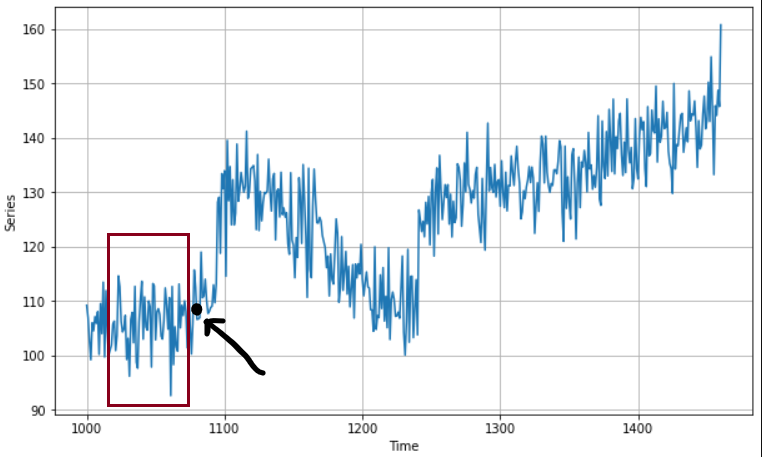
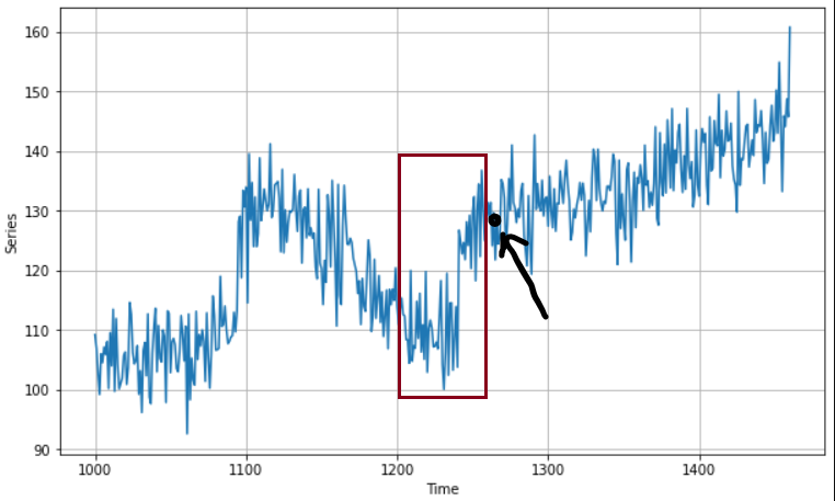
The red box is your window, on whose sequence of values your model will learn and the immediate value outside will be your label (numerical value) to predict.
Let’s prepare the dataset with some code.
The division into Training and Test dataset
split_time = 1000
train_time = time[:split_time]
train_series = series[:split_time]
valid_time = time[split_time:]
valid_series = series[split_time:]
Creating Windows and their label from the dataset using Tensorflow Dataset API
window_size = 20
batch_size = 32
shuffle_buffer_size = 1000
def windowed_dataset(series, window_size,batch_size,shuffle_buffer_size):
    dataset = tf.data.Dataset.from_tensor_slices(series)
    dataset = dataset.window(window_size+1, shift = 1, drop_remainder = True)
    dataset = dataset.flat_map(lambda window: window.batch(window_size+1))
    dataset = dataset.map(lambda window: (window[:-1], window[-1:]))
    dataset = dataset.shuffle(shuffle_buffer_size)
    dataset = dataset.batch(batch_size).prefetch(1)
    return dataset
3. Create a model with just one Neuron
The most basic way to understand and work with any new concept from deep learning is by using only a single neuron and observe its execution. Let us just do that.
First, we will use the function `windowed_dataset` defined above to prepare my training and test data, and then we will create a single neuron model using Tensorflow Sequential API.
l0 = tf.keras.layers.Dense(1, input_shape=[window_size])
model = tf.keras.models.Sequential([l0])
model.compile(loss = 'mse', optimizer = tf.keras.optimizers.SGD(lr = 1e-6, momentum=0.9))
model.fit(dataset, epochs=100)
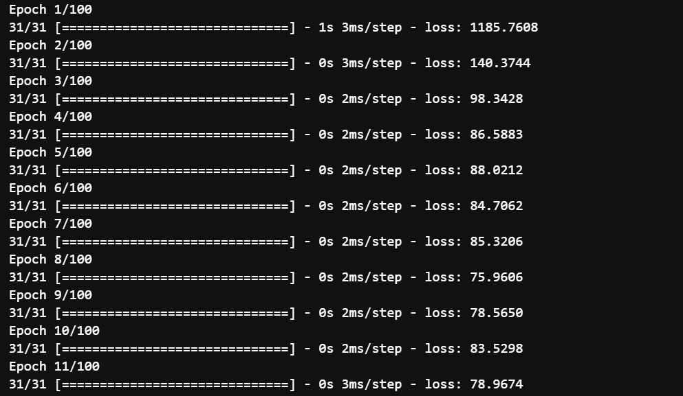
You can clearly see that for a single neuron, it is not bad to reduce the loss from 1185 to 47. It could only do so much. Let us look at how it would perform on the testing set.
TESTING / FORECASTING (in this case)
This method of testing would be slightly different from what you might have done so far. Because we are dealing with sequences and numerical values predicted from the window dataset. We need to save these outputs in a sequence as well. Let’s see how it is done:
forecast = []
for time in range(len(series)-window_size):
  forecast.append(model.predict(series[time:time+window_size][np.newaxis]))
forecast = forecast[split_time-window_size:]
results=np.array(forecast)[:, 0, 0]
NOTE: [np.newaxis] is added to make the data of the same shape the model trained on (1, window_size) and forecast is filtering split_time – window_size because the first value in the testing will come from the output of the last 20(window_size) value from the training. (They were split that way)
Here is how the prediction/ forecast array would look like compared to testing data.
plt.figure(dpi = 120)
plot_series(valid_time, valid_series)
plot_series(valid_time, results)
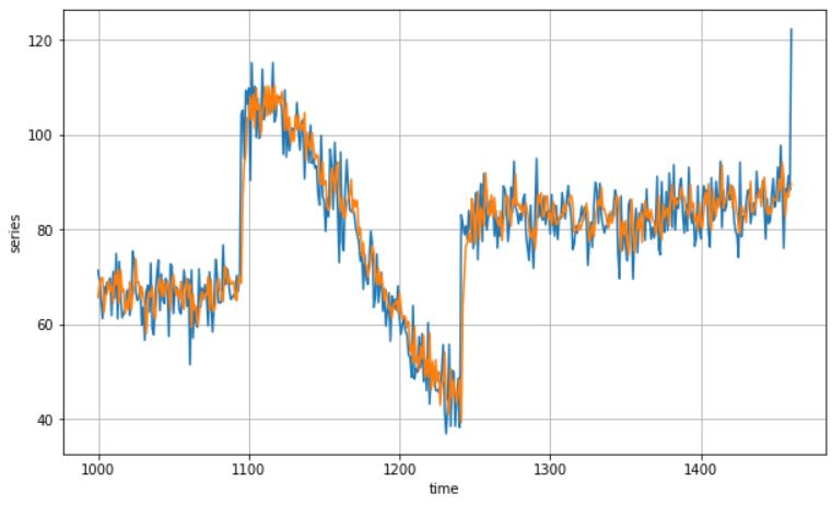
At Last, let’s measure the mean absolute error between the labels and the predictions.
tf.keras.metrics.mean_absolute_error(valid_series, results).numpy()
MAE: 5.2105947
Conclusion: Although you can see a pretty low MAE, that doesn’t mean that this is a very good model because, with one neuron, the model has even learned the noise along with trend and seasonality and also this is a synthetic data, which is mathematically computed so things are similar to as an ideal case. For stronger models, we use neural networks that can work on sequences of data like (recurrent Neural Network and Long Short Term Memory cells (LSTMs) and more)
I hope you enjoyed getting familiar with time series and how common are they in our daily surrounding data. Thank you and that would be it from my side.
Gargeya Sharma
B.Tech Computer Science 4th year
Specialized in Data Science and Deep Learning
Data Scientist Intern at Upswing Cognitive Hospitality SolutionsFor more info check out my Github Home Page
Photo by Nathan Dumlao on Unsplash
The media shown in this article are not owned by Analytics Vidhya and are used at the Author’s discretion.


