This article was published as a part of the Data Science Blogathon
We have dived deep into what is a Neural Network, its structure and components, Gradient Descent, its limitations and how are neurons estimated, and the working of the forward propagation.
Forward Propagation is the way to move from the Input layer (left) to the Output layer (right) in the neural network. The process of moving from the right to left i.e backward from the Output to the Input layer is called the Backward Propagation.
Backward Propagation is the preferable method of adjusting or correcting the weights to reach the minimized loss function. In this article, we shall explore this second technique of Backward Propagation in detail by understanding how it works mathematically, why it is the preferred method. A caution, the article is going to be a mathematically heavy one but wait for the end to see how this method looks in action 🙂

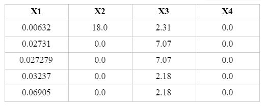
Let’s say we want to use the neural network to predict house prices. For our understanding purpose here, we will take a subset dummy dataset having four input variables and six observations here with the input having a dimension of 4*5:
The neural network for this subset data looks like below:
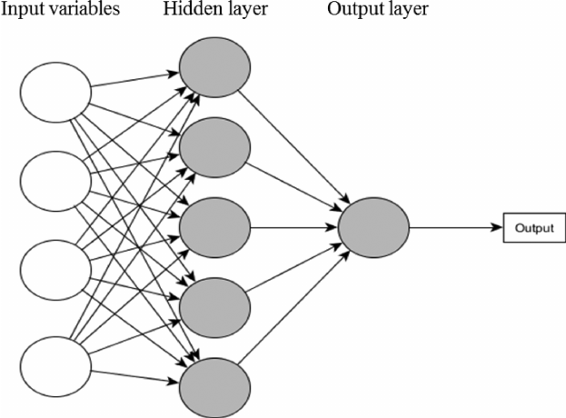
Source: researchgate.net
The architecture of the neural network is [4, 5, 1] with:
A Neural Network operates by:
We repeat these three steps until have reached the optimum solution of the minimum loss function or exhausted the pre-defined epochs (i.e. the number of iterations).
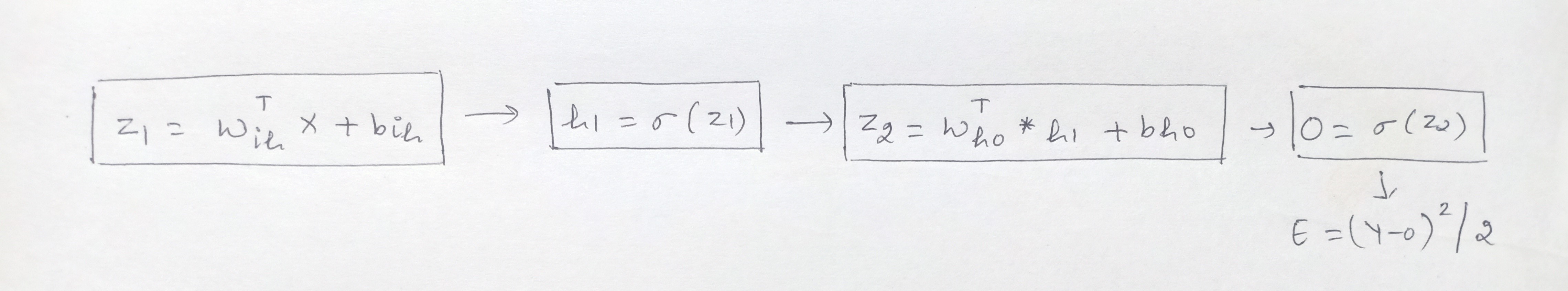
Now, the computation graph after applying the sigmoid activation function is:
In case you are wondering how and from where this equation arrived and why there will be matrix dimensions then request you to read the previous article to understand the mechanism of how neural networks work and are estimated.
Building on this, the first step in Backward Propagation to calculate the error. In our regression problem, we shall take the loss function = (Y-Y^)2/2 where Y is actual values and Y^ is predicted values. For simplicity, replacing Y^ with O, so the error E becomes = (Y-O)2/2.
Our goal is to minimize the error that is clearly dependent on Y, which is the actual observed values, and on the output, which is further is dependent on the:
Now, we can neither change the input variables nor the actual Y values however, we can change the other factors. The activation function and the optimizers are the tuning parameters – and we can change these based on our requirement.
The other two factors: the coefficients or betas of the input variables (Wis) and the biases (bho, bih) are updated using the Gradient descent algorithm with the following equation:
Wnew = Wold – (α * dE/dW)
where,
In the backward propagation, we adjust these weights or the betas in the output. The weights and biases between the respective input, hidden and output layers we have here are Wih, bih, Who, and bho:
In the first iteration, we randomly initialize the weights. In the second iteration, we change the weights of the hidden layer that is closest to the output layer. In this case, we go from the output layer, hidden layer, and then to the input layer.
Now, we have to calculate how much each of these weights (Wis) and biases (bis) contribute to the error term. For this, we need to calculate the rate of change of error to the respective weights and bias parameters.
In other words, we need to compute the terms: dE/dWih, dE/dbih, dE/dWho, and dE/dbho. This is not a direct task. It is a series of steps involving the Chain Rule.
The weight, Who, between the hidden and the output layer:
From the above graph we can see that the error E is not directly dependent on the Who:
Therefore we employ the chain rule to compute the rate of change in error to the change in weight Who and it becomes:
dE/dWho = dE/dO * dO/dZ2 * dZ2/dWho
Now, we take the partial derivatives of each of these individual terms:
E = (Y-O)2/2.
The partial derivative of error with respect to Output is: dE/dO = 2*(Y-O)*(-1)/2 = (O-Y)
The partial derivative of Output with respect to Z2, as output O = Sigmoid of Z2 and the derivative of sigmoid is:
dO/dZ2 = sigmoid(Z2) *(1-sigmoid(Z2)) = O*(1-O)
The partial derivative of Z2 with respect to Who is:
dZ2/dWho = d(WhoT * h1 + bh0)/dWho
dZ2/dWho = d(WhoT * h1)/dWho + d(bho/Who) = h1 + 0 = h1
Therefore, dE/dWho = dE/dO * dO/dZ2 * dZ2/dWho becomes:
dE/dWho = (O-Y) * O*(1-O) * h1
Similarly, we will calculate the contribution for each of the other parameters in this manner.
For the bias, bho, between the hidden and the output layer:
dE/dbho = dE/dO * dO/dZ2 * dZ2/dbho
dE/dbho = (O-Y) * O*(1-O) * 1
The weight, Wih, between the input and the hidden layer:
From the above graph we can see that the terms are dependent as below:
dE/dWih = dE/dO * dO/dZ2 * dZ2/dh1 * dh1/dZ1 * dZ1/dWih
So, this time, apart from the initial above dE/dO, dO/dZ2, we have the partial derivatives as follow:
The partial derivative of Z2 with respect to h1 is:
dZ2/dh1 = d(WhoT * h1 + bho)/dh1
dZ2/dh1 = d(WhoT * h1)/dh1 + d(bho/h1) = Who + 0 = Who
The partial derivative of h1 with respect to Z1, as h1 = Sigmoid of Z1 and the derivative of sigmoid is:
dh1/dZ1 = sigmoid(Z1) *(1-sigmoid(Z1)) = h1* (1 – h1)
The partial derivative of Z1 with respect to Wih is: X
dZ1/dWih = d(WihT * X + bih)/dWih
dZ1/dWih = d(WihT * X)/dWih + d(bih/Wih) = X + 0 = X
Hence, the equation after plugging the partial derivative value is:
dE/dWih = dE/dO * dO/dZ2 * dZ2/dh1 * dh1/dZ1 * dZ1/dWih
dE/dWih = (O-Y) * O*(1-O) * Who * h1(1-h1) * X
The bias, bih, between the input and the hidden layer:
dE/dbih = dE/dO * dO/dZ2 * dZ2/dh1 * dh1/dZ1 * dZ1/dbih
dE/dbih = (O-Y) * O*(1-O) * Who * h1(1-h1) * 1
Now, that we have computed these terms we can update the parameters using the following respective update equations:
Now, moving to another method to perform backward propagation …
The backward propagation can also be solved in the matrix form. The computation graph for the structure along with the matrix dimensions is:
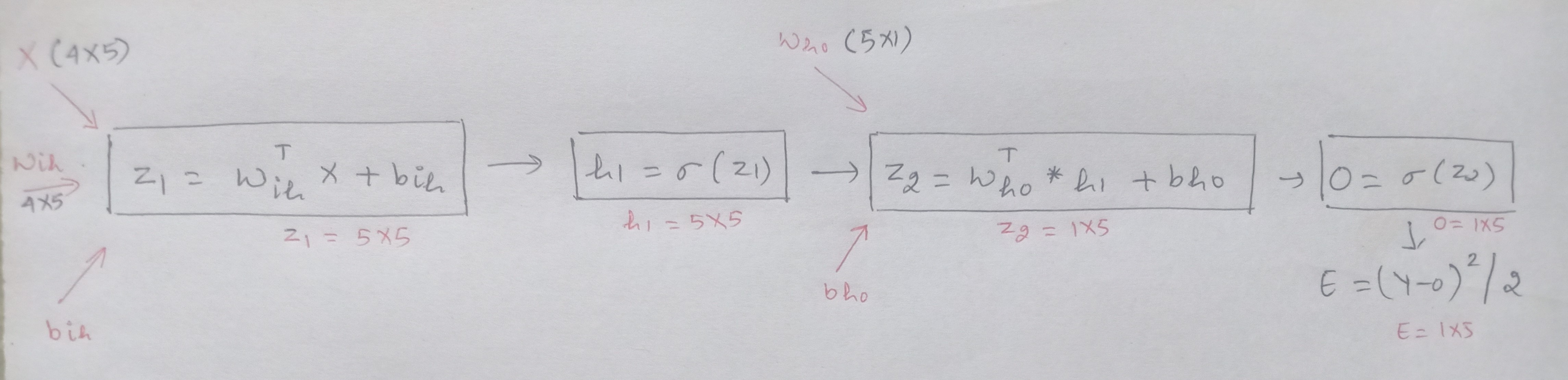
Z1 = WihT * X + bih
where,
Z2 = WhoT * h1 + bho
where,
To summarize, the four equations of the rate of change of error with the different parameters are:
dE/dWho = dE/dO * dO/dZ2 * dZ2/dWho = (O-Y) * O*(1-O) * h1
dE/dbho = dE/dO * dO/dZ2 * dZ2/dbho = (O-Y) * O*(1-O) * 1
dE/dWih = dE/dO * dO/dZ2 * dZ2/dh1 * dh1/dZ1 * dZ1/dWih = (O-Y) * O*(1-O) * Who * h1(1-h1) * X
dE/dbih = dE/dO * dO/dZ2 * dZ2/dh1 * dh1/dZ1 * dZ1/dbih = (O-Y) * O*(1-O) * Who * h1(1-h1) * 1
Now, lets’ see how we can perform matrix multiplication on each of these equations. For the weight matrix between the hidden and the output layer, Who.
Let us understand how the shape of this Who must be similar to that of the shape of dE/dWho, which is to used to update the weight in the following equation:
Who = Who – (α * dE/dWho)
We saw above that dE/dWho is computed using the chain rule and is of the result:
dE/dWho = dE/dO * dO/dZ2 * dZ2/dWho
dE/dWho = (O-Y) * O*(1-O) * h1
Breaking the individual components of this above equation we see each part’s dimension:
dE/dO = (O-Y) as both O and Y have the same shape of 1*5. Hence, dE/dO is of dimension 1*5.
dO/dZ2 = O*(1-O) having a shape of 1*5, and
dZ2/dWho = h1, which is of the shape 5*5
Now, performing matrix multiplication on this equation. As we know, matrix multiplication can be done when the number of columns of the first matrix must be equal to the number of rows of the second matrix. Where this matrix multiplication rule defies, we will take the transpose of one of the matrices to conduct the multiplication.
On applying this our equation takes the form of:
dE/dWho = dZ2/dWho . [dE/dO * dO/dZ2] T
dE/dWho = (5X5) . [(1X5) *(1X5)]T
dE/dWho = (5X5) . (5X1) = 5X1
Therefore, the shape of dE/dWho 5*1 is the same as that of Who 5*1 which will be updated using the Gradient Descent update equation.
In the same manner, we can find perform the backward propagation for the other parameters using matrix multiplication and the respective equations will be:
dE/dWho = dZ2/dWho . [dE/dO * dO/dZ2] T
dE/dbho = dZ2/dbho . [dE/dO * dO/dZ2 ]T
dE/dWih = dZ1/dWih . [dh1/dZ1 * dZ2/dh1. (dE/dO * dO/dZ2)] T
dE/dbih = dZ1/dbih . [dh1/dZ1 * dZ2/dh1. (dE/dO * dO/dZ2)] T
Where, (.) dot is the dot product and * is the element wise product.
To summarize, as promised, below is a very cool gif that shows how backward propagation operates in reaching to the solution by minimizing the loss function or error:

Source: 7-hiddenlayers.com
Backward Propagation is the preferred method for adjusting the weights and biases since it is faster to converge as we move from output to the hidden layer. Here, we change the weights of the hidden layer that is closest to the output layer, re-calculate the loss and if further need to reduce the error then repeat the entire process and in that order move towards the input layer.
Whereas in the forward propagation, the pecking order is from the input layer, hidden, and then to the output layer which takes more time to converge to the optimum solution of the minimum loss function.
I hope the article was helpful to show how backward propagation works. You may reach out to me on my LinkedIn: linkedin.com/in/neha-seth-69771111
Thank You. Happy Learning! 🙂
The media shown in this article are not owned by Analytics Vidhya and are used at the Author’s discretion.
Hi there! I am Neha Seth. I work as a Data Scientist in Larsen & Toubro Infotech (LTI). I hold a Postgraduate Program in Data Science & Engineering from the Great Lakes Institute of Management and a Bachelors in Statistics. I have been featured as Top 10 Most Popular Guest Authors in 2020 on Analytics Vidhya (AV). My area of interest lies in NLP and Deep Learning. I have also passed the CFA Program. You can reach out to me on LinkedIn and can read my other blogs for AV.
Lorem ipsum dolor sit amet, consectetur adipiscing elit,


Thank You for your helpful explanation. I actually made a simple working NN with 2 layers and the training converged. Used Leaky ReLU.