Is Gradient Descent sufficient for Neural Network?

Introduction

An important factor that is the basis of any Neural Network is the Optimizer, which is used to train the model. The most prominent optimizer on which almost every Machine Learning algorithm is built is the Gradient Descent. However, when it comes to building the Deep Learning models, the Gradient Descent has some major challenges.

Before knowing what the issues with Gradient Descent are, the first part of the article is a refresher on how a neural network works and why there is even a need for an optimizer in the first place.

In the second part of the article, we shall dive deep into each of the challenges of Gradient Descent, why these impede the Deep learning model, what are the solutions, and which is the most effective optimizer for the Neural Network.

Table of Contents

• What is a Neural Network?
• How a Neural Network Works?
• Why do we need Optimizers for Neural Networks?
• Challenge 1: Gradient Descent gets stuck at Local Minima
• Stochastic Gradient Descent with Momentum
• Challenge 2: Constant Learning Rate in the Gradient Descent
• RMSProp
• Which Optimizer to Use for Neural Network?
• Summary

What is a Neural Network?

Artificial Neural Networks (ANN) are inspired by Biological or Natural Neural Networks (BNN). The purpose of ANN is to stimulate the functionality of a human brain such that it can mimic and take action as a human brain does. Given that ANN is a replica of the human brain so naturally, the components of ANN are also the same as that of the biological neural network.

A neural network is a set or system of interconnected units where each of the connections has a weight attached to it. These interconnected units are also called neurons. The main building block of a neural network is a Neuron. A neuron is a nerve cell that carries electrical impulses. It is the core working unit of the brain that has the responsibility of transmitting information to every other cell in the body.

The human brain receives information via the five sensory organs, processes that information, based on which takes the decision and eventually action.

ANNs function in a similar manner using the neurons (or nodes) that they possess. The difference between ANN and natural neural networks is how each of these networks receives the information.

BNN receives the information from the sensory receptors whereas the inputs in the ANN are the Xs or the independent variables. That is the information gets stored in the form of features or characteristics and this information then has some weights associated with it.

Why do we have the weights associated with the information or with the Xs? How is this similar to the brain neural network?

Well, let’s say you planned to catch the latest flick, 7 Yards: The Chris Norton Story on Netflix. You may have seen the trailer of the documentary, liked it and then your friend says the movie isn’t good, don’t watch it.

Which piece of information would you give more preference to? To your friend’s review or to the perception that you received about the movie via your senses? Most likely, to your viewpoint as the senses are the most important source via which we perceive the world.

This preference to your assessment of the movie vis-a-vis the friend’s review is what is giving weightage to the information. This coherence and the mapping between BNN and ANN are illustrated below:

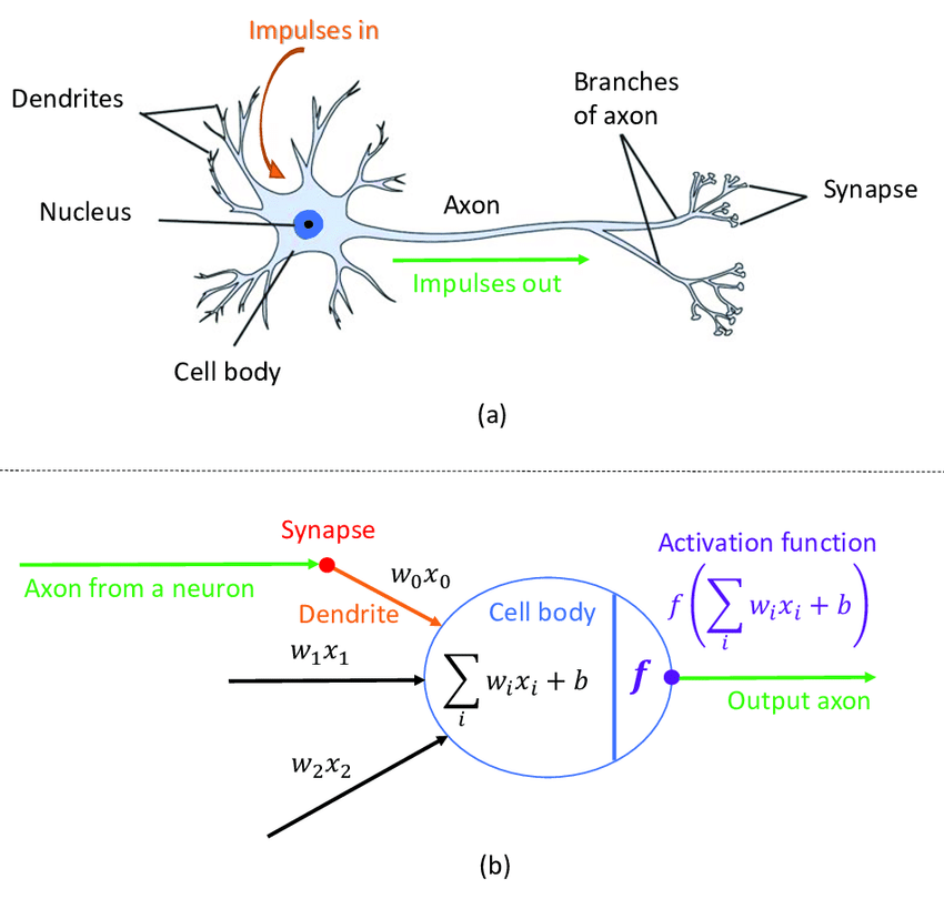
Source: researchgate.net

Now, how does a neural network work? Since the focus of this article is the challenges with Gradient Descent in Neural Networks and the respective solutions, will keep the working of the neural network as succinct as possible yet covering everything that is needed for understanding.

How a Neural Network Works?

We saw above, the neural network consists of inputs, the Xs and there are some weights given to these inputs. And naturally, we’ll have an output of the model. This output depends on the type of business problem we have.

In the case of classifying web pages, it’s a classification problem so then will have multiple classes as the output. Similar to Machine Learning, with ANN or Deep learning as well, the function is a regressor or classifier (binary or multiclass) depending on whether the output variable is continuous or categorical.

Therefore, the architecture of the Neural Network will have at least two layers: the Input and the Output layer. What comes in between these two layers is called the Hidden Layer.

The Hidden Layer consists of the neurons and please note that there are no neurons in the input layer. The input layer only has the inputs, the Xs. Each of these layers is a result of the previous layer and the interconnectivity between each of the layers is shown below:

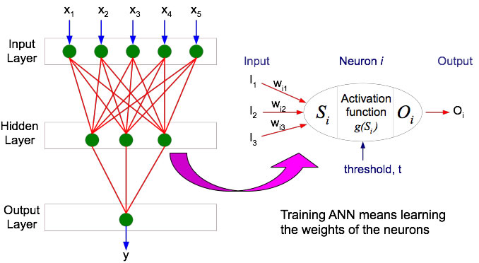
Source: faculty.juniata.edu

There can be any number of hidden layers and any number of neurons in each of the hidden layers. The architecture of the network is defined by the user, hence the number of hidden layers and the number of neurons are at the discretion of the user.

Now, at the end of the day, ANN is an algorithm, so we can’t build any model without having any mathematical equation behind it 🙂 That brings us to how the ANN looks mathematically and what we need to solve it.

The equation is the linear combination of the inputs and their respective weights and a bias term, which is the correction factor having weight as one. The bias term is the intercept, why do we need the intercept term? Because the output of the model can’t be zero if there are no inputs or no independent Xs or features in the model.

To elaborate on that, is it possible for a store to not have any sales if there are no factors such as categories, location, store number? We may not have these details about the store, but if the store exists it is certainly bound to make some sales even if it is a small amount.

So, the neural network equation is:

Z = Bias + W₁X₁ + W₂X₂ + …+ W_nX_n .

Z is the symbol for denotation of the above graphical representation of ANN.

W_is, are the weights or the beta coefficients

X_is, are the independent variables or the inputs

Bias = W₀

Each of the neurons in the hidden layer will have an equation like above which will connect between the layers and the respective weights and the bias terms. This is how the neurons get estimated and then are passed on to the next layer.

Now, if you have been following my previous blogs, by now you know, I like to break into the mathematics behind the concepts. However, concerning the topic of the article, it would not be possible to dive into the estimation process of the neurons here. That’s a different topic on its own. I’ll cover that up in a separate article later.

One more piece in the structure of the neural network before moving to the optimizers is the activation function. The hidden layers, as well as the output layer, are passed through a function called the Activation Function. It is an important part as it adds non-linearity to the function. It is needed because typically not every business problem can be solved linearly. So to take into account the non-linearity, we apply some mathematical transformation to the equation before the output is generated.

In the output layer, the activation function is again based on the type of problem we are dealing with and the activation function on the hidden layers also has some essential properties attached to it. These are shown graphically in the images above.

There are several activation functions and which function to use depends upon their functionality. All we need to know is that the output of the neuron is the output of the activation function.

To summarize, how does a neural network work is:

1. Each of the input-link is assigned a weight. Initially, the weights are randomly assigned. These weights are multiplied by each input value and then added together which results in the following linear combination:

Z = W₀ + W₁X₁ + W₂X₂ + …+ W_nX_n .

2. The above equation is passed through a transformation (the fancy technical word for this transformation is: the Activation or the Squashing function). The activation function depends on the type of data and problem. Hence, it is a tuning parameter for ANN.

For a binary classification problem, we know that Sigmoid is needed to transform the linear equation to a non-linear equation. Therefore, the activation function for binary classification is the Sigmoid and looks like this:

Let says, for neuron 1,

N1 = F(Z)

where Z = W₀ + W₁X₁ + W₂X₂ + …+ W_nX_n which becomes:

N1 = sigmoid(Z)

where, sigmoid(Z) = e^Z/(1+ e^Z)

3. After applying the activation function, the output becomes:

Output = N1

If the transformed equation crosses the threshold for the Neuron then the output is class 1 else the output is class 0.

Okay, so we have a fair understanding of what a neural network is and how it works and this is more than sufficient to understand the role of optimizers in the neural network.

Why do we need Optimizers for Neural Network?

The steps involved in the Neural Network are :

1. We take the input equation:  Z = W₀ + W₁X₁ + W₂X₂ + …+ W_nX_n and calculate the output, which is the predicted values of Y or the Y_pred

2. Calculate the error. It tells how much the model deviates from the actual observed values. It is always calculated as the Y_pred – Y_actual

(Please note which error to calculate changes depending on whether the problem is of regression or classification. For Regression, you can calculate RMSE, MAPE, MAE, and for classification Binary Cross Entropy Cost Function. For more in-depth on the loss function, you may want to refer to this blog.)

3. Up until now, we took the input, found the output, and computed the error term or the loss. Now, if you remember from Machine Learning days, what is the end goal of any model?

It is to minimize this error term! And, how will we do that here in the Neural Network? We take the computed loss value back to each layer so that it updates the weights in such a way that minimizes the loss.

This way of first adjusting the weights or the betas in the output is known as Backward Propagation. On the other hand, the process of going from left to right i.e from the Input layer to the Output Layer for the adjustment of betas is known as the Forward Propagation.

The weights that are referred to here are the same beta coefficients that have been attached to the Xs or the inputs in the input layer.

In short, this last part is what calls forth the powers of optimizers to update the weights. Yay! we finally reached here! 😀

Now let’s build upon this …

The objective of any optimizer is to minimize the loss function or the error term. The loss function gives the distance of the observed value from the predicted value. A loss function must have two qualities: it must be continuous and differentiable at each point. To minimize the loss generated from any model, we need two things:

1) The magnitude that is by how much amount to decrease or increase, and

2) The direction in which to move

Gradient Descent has been doing a fairly good job in helping with these two necessities. How Gradient Descent helps is:

Source: miro.medium.com

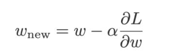
Using Gradient Descent, we get the formula to update the weights or the beta coefficients of the equation we have in the form of  Z = W₀ + W₁X₁ + W₂X₂ + …+ W_nX_n .

W_new = W_old – (α * dL/dw)

where,

W_new = the new weight of Xi

W_old = the old weight of the Xi

α = learning rate

dL/dw is the partial derivative of the loss function for each of the Xs. It is the rate of change of the loss function to the change in weight.

Learning rate and dL/dw help us with the two requirements to minimize the loss function:

• Learning rate: answers the magnitude part. It controls the update of the weights by telling how much amount to increase or decrease.

• dL/dw: conveys how much the parameter must increase or decrease. It indicates the direction by its sign.

It is an iterative process to find the parameters (or the weights) that converge with the optimum solution. The optimum solution is where the loss function is minimized.

Now, as we know there can be numerous hidden layers and neurons in a neural network. We aren’t looking at one specific weight for a single equation. But, the weights attached to each neuron in each layer and that too from the output layer back to the original input layer. In such case, the weights that are updated via Gradient Descent shortfall at two important places:

• Gradient Descent gets stuck at Local Minima
• The learning rate does not change in Gradient Descent

Why is that so and what are the remedies is what all the rest of the article is about.

Challenge 1: Gradient Descent gets stuck at Local Minima

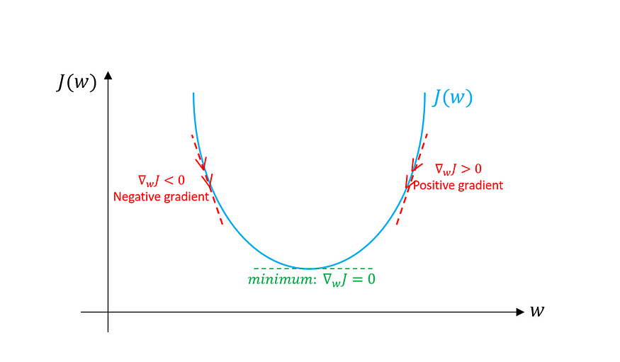
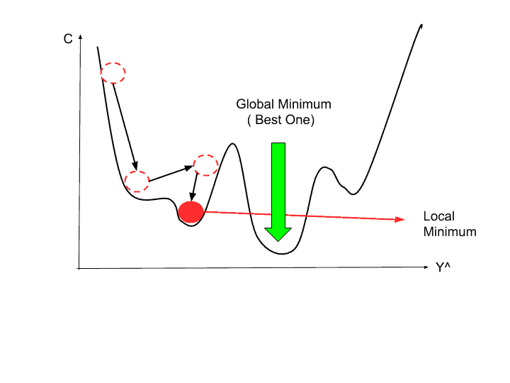
The first challenge with the Gradient Descent is that it gets stuck at the local minima. Let’s understand this by seeing the below cost function.

The pointer with the green arrow is the Global Minima, which is the point where the cost function is the lowest in the entire cost function.

The point where the red ball is placed has minimum cost function value amongst its neighbors and therefore is the Local Minima or the local minimum point. Typically, the gradient descent gets stuck at this point. However, the local minima are not where the cost function is the lowest.

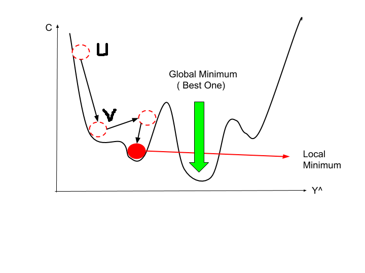
Source: mltut.com

How does Gradient Descent get stuck at the local minima?

In the above visual apart from the red ball, there are three lined red circles as well. At each of these points, we calculate the gradient or the slope and using the below formula to update weights and reduce the cost function.

Now, after a few iterations, we have reached the point where the red ball is placed. At this point, we calculate again and the gradient or slope here is zero and then the equation reduces to:

W_new = W_old

because dL/dw (slope) = 0 which makes the new and past weights as same, and hence, the parameters will not update.

So, once we are stuck at the local point, we need some kind of push to get out of this and move further to reach the global minimum. How do we get that push and ensure we reach the global minima?

The solution to Challenge 1: Stochastic Gradient Descent with Momentum

In the above graph itself, when the ball descends from Position U, it will have some speed, and let’s call that speed as U. Rolling down, the ball has reached position V where the speed is denoted by V based on its position. Now, the speed V will certainly be more than the speed U as the ball is moving in a downward direction.

Now, when the ball has reached the local minima, it would have gained some momentum or the speed which will give the ball the needed push to eventually come out of the local minima. In short, to get the ball out of the local minima, we need accumulating momentum or speed.

How do we represent this mathematically?

In terms of Neural Network, the accumulated speed is equivalent to the weighted sum of the past gradients and this is represented as below:

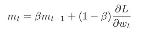
where,

dL/dw = current gradient at the time t

m_t-1 = previously accumulated gradient till the time t-1

ꞵ gives how much weightage to be given to the current gradient and the previously accumulated gradient. Generally, 10 percent weightage is given to the current gradient and 90 percent to the previously accumulated gradient.

So, when at the local minima at the position of the full red ball, the slope dL/dw will be zero and now the equation will become:

m_t = ꞵ*m_t-1

This time the new weights are not equal to the past weights because m_t-1, which is the previously accumulated gradient, has some past value. Therefore, the current weighted m_t will have some value then that will give the required push to come out of the local minima.

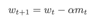
m_t is the new gradient. It is the sum of the current gradient dL/dw at the time t  and of the previously accumulated gradient m_t-1till the time t-1.

m_t is now used to update the weights to minimize the cost function for the Neural Network using the equation:

Moving on to the next issue with Gradient Descent …

Challenge 2: The learning rate does not change in Gradient Descent

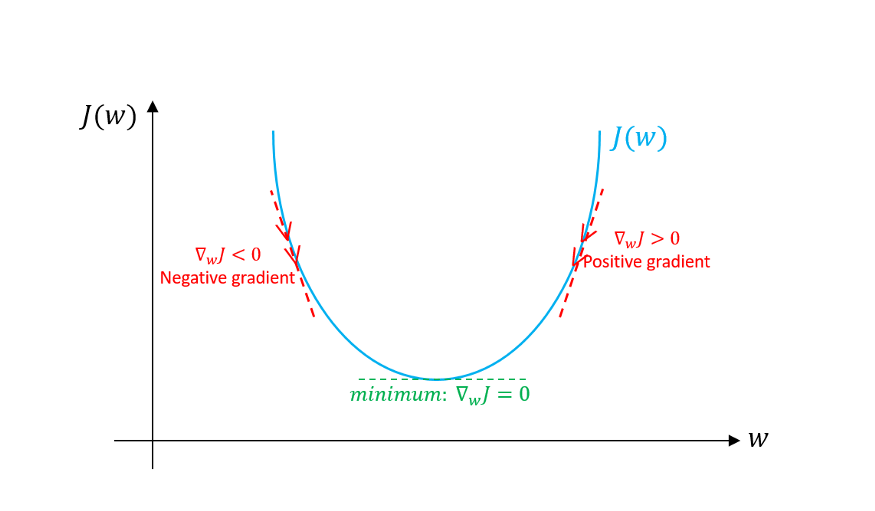
The second problem with Gradient Descent is that the learning rate remains the same throughout the training process for all the parameters. To recall, the learning rate is the step size that specifies to the algorithm how much it must make to reach the optimal solution of the minimized error term.

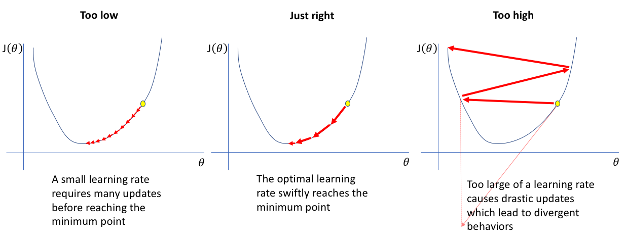
Source: www. jeremyjordan. me

In general, some variables may lead to faster convergence than the other variables. By using a constant learning rate throughout the training process, we may be forcing those variables to remain in sync and leading to slower convergence to the optimal solution.

So, we want that the learning rate is updated as per the cost function as the training progresses. How can we do this?

The solution to Challenge 2: RMSProp

During the training process, the slope or the gradient dL/dw changes. It is the rate of change in the loss function concerning the parameter weight and by applying this we can update the learning rate.

We can take the sum of squared the past gradients i.e square of the sum of the partial derivatives of dL/dw as below:

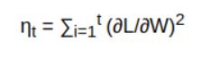
The reason we take the square of these gradients is to eliminate the effect as some of the gradients will be positive and some will be negative. That tends to nullify the result. Hence, we take the square of the gradients and add it to the past squared slopes which are represented by η.

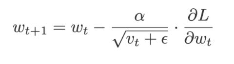
Using η can update the learning rate in the following equation i.e is used to calculate the new weights:

W_new = W_old – (α /√η) * (dL/dw)

Now, comes the catch! We have squared the slopes, which is needed to remove the cancellation effect due to the signs. However, the square of any number is always positive, and adding these slopes will always increase the η.

On using η to scale the learning rate, will always decrease the second part of the above equation: (α /√η) * (dL/dw) because η is in the denominator. Also, note we are taking the root of η.

Over time with iterations, the learning rate will become infinitely small and this part will tend to zero. It will eventually make the W_new ~= W_old and will lead to slower convergence to the optimum solution.

So, how do we deal with this issue now?

We employ η in the equation of the weighted sum of gradients, which we used to resolve the first challenge of Gradient Descent to get out of the local minima:

As we just saw, we’ll use the square of the slopes, so plugging that into this equation will become:

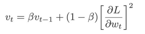
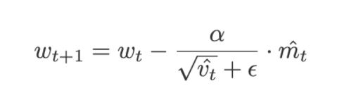
Now using, the weighted sum of the squared past gradients, the equation to update the new weights become:

where,

ε is the error term. It is added to V_t so that the denominator does not become zero and this error term is generally very small in value.

Let’s understand how does this final equation help in updating the learning rate during the training process:

• When the square of the slopes is high i.e (dL/dw)², then this will increase the value of V_t and which would reduce the learning rate.
• Similarly, the value of V_t will be low when the square of the slopes is low i.e (dL/dw)², and this will increase the learning rate.

Visually can see in the graph below: in the left panel, the loss value on the function is at the first topmost point. At this point, we will calculate the gradient. Here, the magnitude of the slope is high, which will also increase the square of the slope. This will reduce the learning rate and we must take small steps to minimize the loss. The small steps are illustrated by the downward steps on the loss function.

Source: cms

Whereas, the graph on the right side, where the lowest point on the loss function has a low magnitude of the gradient. Therefore, the square of this gradient will also be less. It will increase the learning rate and hence will take bigger steps towards the optimal solution.

This is how the RMSProp scales the learning rate depending on the square of the gradients, which eventually leads to faster convergence to the optimal solution.

Which Optimizer to Use for Neural Network?

Now, we have seen the above two solutions where Stochastic Gradient Descent with Momentum helps with the problem of getting stuck at the local minima and RMSProp changes the learning rate as per the cost function.

So, which optimizer shall we use to train the Neural Network? Do we have to choose between the two or is there a way to combine both of these optimizers? Ask and you shall receive!

There is another breed of the optimizer (Oh yeah! there are tons of optimizers available out there for Neural Networks!). The optimizer on which we’ll focus that resolves both the problems of Gradient Descent is called Adam.

Adaptive Moment Estimation (or Adam) is the blend of the Stochastic Gradient Descent with Momentum and RMSProp. It is the most popular and the most effective of all the optimizers.

From Stochastic Gradient with Momentum and RMSProp, we have:

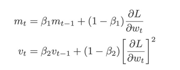
The weight update equation for Adam becomes:

Summary

The two problems with the Gradient Descent are:

1. The Gradient Descent gets stuck at the local minima. The solution for this is using Stochastic Gradient with Momentum, which uses the weighted sum of gradients to help to get out of the local minima.

2. The learning rate in Gradient Descent is constant throughout the training process for all the parameters. This can slow the convergence. As the remedy for this, we change the optimizer from Gradient Descent to RMSProp.

Using the weighted sum of the squared past gradients, RMSProp changes the learning rate according to the cost function that leads to faster convergence to the optimal solution of minimizing the error.

Adaptive Moment Estimation (or Adam) provides the benefits of both the Stochastic Gradient Descent with Momentum and RMSProp.

I hope this article was helpful to know about the Neural Networks, the need for Optimizers in Neural Networks, the challenges with Gradient Descent, and how it can be resolved.

You may reach out to me on my LinkedIn: linkedin.com/in/neha-seth-69771111

Thank You. Happy Learning 🙂

Neha

Hi there! I am Neha Seth. I work as a Data Scientist in Larsen & Toubro Infotech (LTI). I hold a Postgraduate Program in Data Science & Engineering from the Great Lakes Institute of Management and a Bachelors in Statistics. I have been featured as Top 10 Most Popular Guest Authors in 2020 on Analytics Vidhya (AV).

My area of interest lies in NLP and Deep Learning. I have also passed the CFA Program. You can reach out to me on LinkedIn and can read my other blogs for AV.