This article was published as a part of the Data Science Blogathon
Objective
From this article, you will learn how to predict the monthly sales of all different items at different shops, given the historical daily sales data (with code!).

It is an integral part of the business to make an intelligent business decision to save cost or gain more profit. Good forecasting can help to ensure the retailers maintain adequate inventory levels, mitigate the chance of stock obsolete, or supply the right product at the right time and location. For example, if the forecast indicates a 25% increase in sales of products or services, the store can purchase those products ahead to meet the demand. Conversely, a forecast of shortfalls in sales can allow people to mitigate the effect by taking actions ahead.
Challenges of the problem
Build a good model from observed time series data is challenging because time series data are usually unstable and continuous. For instance, future sales can be affected by new products launch, promotions available, seasonality, and other changes that make it very difficult to predict using past behaviors. Furthermore, there is only a single historical sample available in each data instance, hence, we might need to add lag terms to perform the forecasting task.
Dataset Description
The dataset can be downloaded from here. The definition of data files and fields are as follow:
sales_train.csv – training dataset. Daily historical data from January 2013 to October 2015.
- date – date in format dd/mm/yyyy
- date_block_num – a consecutive month number, used for convenience. January 2013 is 0, February 2012 is 1, …, October 2015 is 33.
- shop_id – unique identifier of a shop
- item_id – unique identifier of a product
- item_price – the current price of an item
- item_cnt_day – number of products sold per day
test.csv – test dataset. The task is to predict total sales for every item and shop in the next month i.e. November 2015 which date_block_num is 34.
- Id – represents a (shop, item) tuple within the test set
- shop_id – unique identifier of a shop & item_id – unique identifier of a product
item_categories.csv – information about the items’ categories.
- item_category_id – unique identifier of the item category
- item_category_name – the name of the item category
shops.csv – information about the shops.
- shop_id – unique identifier of a shop
- shop_name – the name of shop
items.csv – information about the items or products.
- item_category_id – unique identifier of the item category
- item_id – unique identifier of a product
- item_name – the name of the item
Data Cleaning
1. Checking missing values: There are no missing values in all the data files mentioned above.
2. Remove outliers: removing the noisy data values/obvious outliers by defining some threshold.
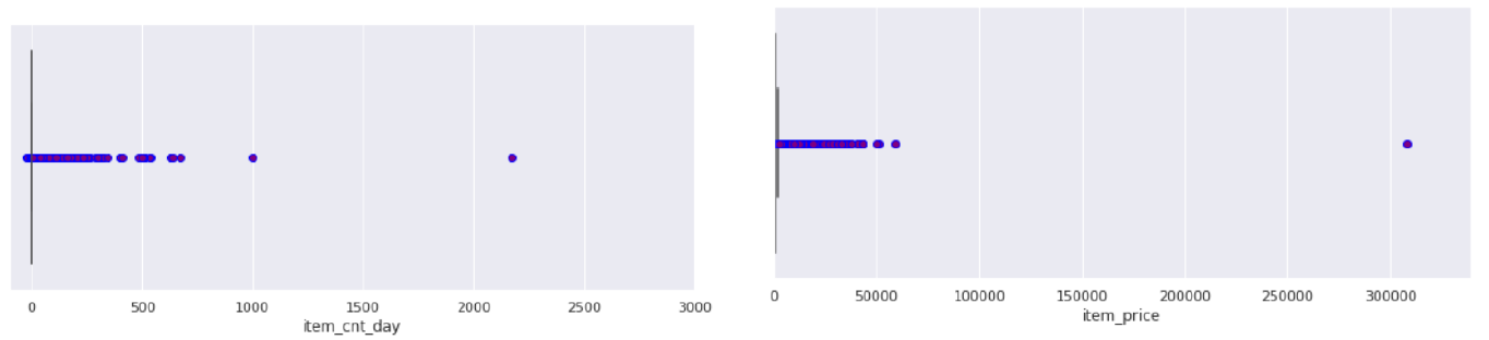
Defined threshold:
- item_cnt_day – remove the data instances that sold more than 1500 in one day.
- item_price – remove the item with a price greater than 150,000.
3. Remove data instances with negative price or item count: Remove any data instances where the item price or item_cnt_day values are negative. These data points might be due to the refund. But for simplicity, I decided to remove those data points.
4. Combine duplicated feature values into a single feature value: several shops seems to be the same to each other. This could be possibly due to moving store locations or shops re-opening. For instance, shop name “!Якутск Орджоникидзе, 56 фран” and “Якутск Орджоникидзе, 56” are being treated as the same shop after pre-processing.
5. Feature construction: construct a new feature to capture important information.
- shop_name’s feature values represent both the shop location (city) and shop category (i.e. shopping center, outlet, etc). Therefore, I have created 2 new features named “shop_city” and “shop_category”. Further aggregate shop category feature values by only keeping shop category if there are 5 or more shops of that category and the rest are grouped as “other”.
- item_category_name’s feature values can further break down into category and subcategory. For instance, Accessories – PS4 is split into “Accessories” as a category and “PS4” as a subcategory.
- Since the objective is to predict monthly sales, it is needed to create the “item_cnt_month” feature by summing up all the “item_count_day” for specific shop and item within a month.
- Create “revenue” feature by multiplying “item_cnt_month” and “item_price”
- Split the date feature into “month” and “days”
- “previousMth_avg_item_cnt” by averaging all the “item_cnt_month” of the previous month. In other words, it means an average number of items sold in the previous month.
- “shopSubcategory_avg_item_cnt” by averaging all “item_cnt_month” for each shop and each item subcategory combinations within a month.
- “shopCity_avg_item_cnt” by averaging all “item_cnt_month” for each city within a month.
- “shopCityItem_avg_item_cnt” by averaging all “item_cnt_month” for each city and each item combinations within a month.
- “item_avg_item_cnt” by averaging all the “item_cnt_month” for each item within a month.
- “shop_avg_item_cnt” by averaging all the “item_cnt_month” for each shop within a month.
- “shopItem_avg_item_cnt” by averaging all the “item_cnt_month” for each item and each shop combinations within a month.
- Create side features called “globalAvg_item_price” and and “shop_avg_item_price” to calculate for “delta_price”. “globalAvg _item_price” is the average item price of each item for a whole time frame of 33 months, “shop_avg_item_price” is the average item price of each item within a month, “delta_price” is the difference between “avg_item_price” and “shop_avg_item_price”. This “delta_price” is aimed to capture how the current month’s average item price is related to the global average item price.
- Create side features called “globalAvg_shop_revenue” and and “shop_avg_revenue” to calculate for “delta_revenue”. “globalAvg_shop_revenue” is the average revenue of each shop for a whole time frame of 33 months, “shop_avg_revenue” is the average revenue of each store within a month, “delta_revenue” is the difference between “globalAvg_shop_revenue” and “shop_avg_revenue”. This “delta_revenue” is aimed to capture how current month average shop revenue is related to global average shop revenue.
Since time series data is non-stationary, the differencing features “delta_price” and “delta_revenue” is a transformation that could somehow help to stabilize or reduce the effect of trend and seasonality.
6. Add lag features: a time series is a sequence of observations taken sequentially in time. In order to predict time series data, the model needs to use historical data then using them to predict future observations. The steps that shifted the data backward in time sequence are called lag times or lags. Therefore, a time series problem is usually transformed into a supervised machine learning problem adding lags as input features.
- Add 3 steps back in time; 3-lags for “item_cnt_moth” feature
- Add 3 steps back in time; 3-lags for “item_avg_item_cnt” feature
- Add 3 steps back in time; 3-lags for “shop_avg_item_cnt” feature
- Add 3 steps back in time; 3-lags for “shopItem_avg_item_cnt” feature
Combine all the features generated in step 5. and create a dataframe with every combination of (month, shop, and item) of increasing month order. After that delete the first 3 months’ data instances from the dataframe since they don’t have lag values.
7. Label Encoding: All the categorical variables in my dataset such as category, sub_category, and shop_city have no order. However, I am using label encoding instead of one-hot encoding because I am going to use a tree-based model (XGBRegressor) which will pick a random set of features to split the tree based on how well that splitting will result in purify child nodes.
Experiments
ML Model
The model I am going to use is the eXtreme Gradient Boosting Regressor aka XGBRegressor. It is particularly popular because it has been the winning algorithm in several recent Kaggle competitions. It is an ensemble learning method that will create a final model by combining several weak models.
As described in the name gradient boosting machine use gradient descent and boosting method. Boosting method adopts the iterative procedure to adaptively change the distribution of training data by focusing more on previously misclassified records to build the base learners. It can be considered as adding the models sequentially until no further improvement is made. A gradient descent algorithm is used to minimize the loss. In gradient boosting where the predictions of multiple models are combined the gradient is used to optimize the boosted model prediction in each boosting round.
XGBoost is a special implementation of a gradient boosting machine that uses more accurate approximations to find the best model. It improves upon gradient boosting machine framework through systems optimization and algorithmic enhancements. Some of its improvements are computing second-order gradients which need fewer steps to coverage to the optimum and regularization terms which improve model generalization.
Train-val-test split
Since I am dealing with a time series dataset, splitting the data randomly will lead to the wrong prediction. Therefore, I have selected the first 4 to 32 months of data as training dataset, month 33 as validation data, and month 34 as testing data. Next, I am going to train the model using train data and tune hyperparameters using the validation set.
Training and Tuning hyperparameters
- Before performing hyperparameter tuning, I have set the “n_estimators” = 1000 and “early_stopping_rounds” = 20 which are used to determine the optimal number of boosting rounds. Furthermore, I have also fixed the eta = 0.1.
- early_stopping_rounds: it will stop training if the error stops reducing for a specific threshold.
- n_estimators: corresponds to the maximum number of boosting rounds or number of gradient boosted trees to build. Usually set it to a large value and together with early_stopping_rounds threshold to find the optimal number of rounds before reaching it.
- eta: parameter the control the learning rate. If the learning rate is high, it is difficult to converge. On the other hand, if the learning rate is too low it will take more boosting round to converge.
I have chosen 5 of the hyperparameters that are usually having a high impact on performance; “max_depth”, “min_child_weight”, “subsample”, “cosample_bytree”, and “alpha”. The evaluation metric used to train the model is the root mean squared error (RMSE).
- max_depth: maximum tree depth for base learners. The deeper the tree, the more complex the model. However, if the tree is too deep, the split becomes less relevant and will cause the model to overfit. A set of 4 candidate values {5, 9, 10, 14}
- min_child_weight: corresponds to a minimum number of instances needed to be in each node. A smaller min_child_weight will lead to a child node with fewer samples and thus allowing a more complex tree. A set of 4 candidate values {1, 5, 6, 10}
- subsample: subsampling ratio of the training instances. It will occur once in every boosting iteration. Subsample ratio = 0.5 means that the algorithm would randomly sample half of the training data prior to growing trees. A set of 4 candidate values {1, 0.8, 0.6, 0.3}
- cosample_bytree: subsample ratio of columns or features when constructing each tree. Similarly, it occurs once in every boosting iteration. Colsample_bytree = 1 means that we will use all features. A set of 4 candidate values {1, 0.8, 0.6, 0.3}
- alpha: L1 regularization parameters to avoid overfitting or control model complexity. A set of 4 candidate values {0.05, 0.1, 0.2, 0.3, 0.5}
The total combinations using the above hyperparameters will need to run 4x4x4x4x5 = 1280 different models. With limited time and computational resources, I have decided to run these hyperparameters in pairs, i.e. first performed hyperparameter tuning using a combination of max_depth and min_child_weight, second performed using combinations of subsample and cosample_bytree, third performed on alpha, and finally performed on eta.
Results
Table 1: The performance on the training set and validation set by varying values of max_depth and min_child_weight in XGBRegressor (in RMSE)
| RMSE on training set | RMSE on validation set | |
| max_depth = 5, min_child_weight = 1 | 0.85729 | 0.90985 |
| max_depth = 5, min_child_weight = 5 | 0.85209 | 0.90801 |
| max_depth = 5, min_child_weight = 6 | 0.84928 | 0.90789 |
| max_depth = 5, min_child_weight = 10 | 0.84632 | 0.90671 |
| max_depth = 9, min_child_weight = 1 | 0.80990 | 0.89646 |
| max_depth = 9, min_child_weight = 5 | 0.78785 | 0.89408 |
| max_depth = 9, min_child_weight = 6 | 0.80670 | 0.89383 |
| max_depth = 9, min_child_weight = 10 | 0.80193 | 0.89292 |
| max_depth = 10, min_child_weight = 1 | 0.78412 | 0.89490 |
| max_depth = 10, min_child_weight = 5 | 0.76146 | 0.89195 |
| max_depth = 10, min_child_weight = 6 | 0.78534 | 0.89334 |
| max_depth= 10, min_child_weight= 10 | 0.75548 | 0.89255 |
| max_depth = 14, min_child_weight = 1 | 0.67286 | 0.89773 |
| max_depth = 14, min_child_weight = 5 | 0.72487 | 0.89512 |
| max_depth = 14, min_child_weight = 6 | 0.72679 | 0.89628 |
| max_depth= 14, min_child_weight= 10 | 0.71907 | 0.89314 |
We get the best score with max_depth = 10 and min_child_weight = 5.
Table 2: The performance on the training set and validation set by varying values of subsample and cosample_bytree in XGBRegressor (in RMSE)
| RMSE – training set | RMSE – validation set | |
| subsample = 1, cosample_bytree = 1 | 0.77881 | 0.89499 |
| subsample = 1, cosample_bytree = 0.8 | 0.80461 | 0.89839 |
| subsample = 1, cosample_bytree = 0.6 | 0.77588 | 0.89328 |
| subsample = 1, cosample_bytree = 0.3 | 0.79709 | 0.89300 |
| subsample = 0.8, cosample_bytree = 1 | 0.77680 | 0.89501 |
| subsample = 0.8, cosample_bytree = 0.8 | 0.76146 | 0.89195 |
| subsample = 0.8, cosample_bytree = 0.6 | 0.77924 | 0.89056 |
| subsample = 0.8, cosample_bytree = 0.3 | 0.79472 | 0.88637 |
| subsample = 0.6, cosample_bytree = 1 | 0.79843 | 0.89901 |
| subsample = 0.6, cosample_bytree = 0.8 | 0.78591 | 0.90145 |
| subsample = 0.6, cosample_bytree = 0.6 | 0.77927 | 0.88560 |
| subsample = 0.6, cosample_bytree = 0.3 | 0.79306 | 0.88662 |
| subsample = 0.3, cosample_bytree = 1 | 0.79265 | 0.89602 |
| subsample = 0.3, cosample_bytree = 0.8 | 0.81131 | 0.89944 |
| subsample = 0.3, cosample_bytree = 0.6 | 0.79335 | 0.89067 |
| subsample = 0.3, cosample_bytree = 0.3 | 0.78281 | 0.88789 |
We get the best score with subsample = 0.6 and cosample_bytree = 0.6.
Table 3: The performance on
training set and validation set by varying values of alpha in XGBRegressor (in RMSE)
| RMSE – training set | RMSE – validation set | |
| alpha = 0.5 | 0.77921 | 0.89105 |
| alpha = 0.3 | 0.77943 | 0.88729 |
| alpha = 0.2 | 0.78550 | 0.89182 |
| alpha = 0.1 | 0.77927 | 0.88560 |
| alpha = 0.05 | 0.78821 | 0.89116 |
We get the best score with alpha = 0.1
Here is what the final models’ parameters looks like:
model = XGBRegressor (max_depth = 10,
                                            n_estimators = 1000,
                                            min_child_weight = 5,
                                            subsample = 0.6,
                                           cosample_bytree = 0.6,
                                           alpha = 0.1,
                                           eta = 0.1,
                                           seed = 42)
Codes
import numpy as np
import pandas as pd
import matplotlib.pyplot as plt
import seaborn as sns
sns.set(style="darkgrid")

# load data
items=pd.read_csv("/kaggle/input/competitive-data-science-predict-future-sales/items.csv")
shops=pd.read_csv("/kaggle/input/competitive-data-science-predict-future-sales/shops.csv")
cats=pd.read_csv("/kaggle/input/competitive-data-science-predict-future-sales/item_categories.csv")
train=pd.read_csv("/kaggle/input/competitive-data-science-predict-future-sales/sales_train.csv")
test=pd.read_csv("/kaggle/input/competitive-data-science-predict-future-sales/test.csv")

# Data Cleaning
plt.figure(figsize=(10,4))
plt.xlim(-100, 3000)
flierprops = dict(marker='o', markerfacecolor='purple', markersize=6,
                  linestyle='none', markeredgecolor='black')
sns.boxplot(x=train.item_cnt_day, flierprops=flierprops)

plt.figure(figsize=(10,4))
plt.xlim(train.item_price.min(), train.item_price.max()*1.1)
sns.boxplot(x=train.item_price, flierprops=flierprops)

# Remove outlier
train = train[(train.item_price < 300000 )& (train.item_cnt_day < 1000)]
# remove negative item price
train = train[train.item_price > 0].reset_index(drop = True)

# Cleaning shops data
# Якутск Орджоникидзе, 56
train.loc[train.shop_id == 0, 'shop_id'] = 57
test.loc[test.shop_id == 0, 'shop_id'] = 57
# Якутск ТЦ "Центральный"
train.loc[train.shop_id == 1, 'shop_id'] = 58
test.loc[test.shop_id == 1, 'shop_id'] = 58
# Жуковский ул. Чкалова 39м²
train.loc[train.shop_id == 10, 'shop_id'] = 11
test.loc[test.shop_id == 10, 'shop_id'] = 11

# Clean up some shop names and add 'city' and 'category' to shops df.
shops.loc[ shops.shop_name == 'Сергиев Посад ТЦ "7Я"',"shop_name" ] = 'СергиевПосад ТЦ "7Я"'
shops["city"] = shops.shop_name.str.split(" ").map( lambda x: x[0] )
shops["category"] = shops.shop_name.str.split(" ").map( lambda x: x[1] )
shops.loc[shops.city == "!Якутск", "city"] = "Якутск"

# Only keep shop category if there are 5 or more shops of that category, the rest are grouped as "other".
category = []
for cat in shops.category.unique():
    if len(shops[shops.category == cat]) >= 5:
        category.append(cat)
shops.category = shops.category.apply( lambda x: x if (x in category) else "other" )

# label encoding
from sklearn.preprocessing import LabelEncoder
shops["shop_category"] = LabelEncoder().fit_transform( shops.category )
shops["shop_city"] = LabelEncoder().fit_transform( shops.city )
shops = shops[["shop_id", "shop_category", "shop_city"]]

# Cleaning Item Category Data
cats["type_code"] = cats.item_category_name.apply( lambda x: x.split(" ")[0] ).astype(str)
cats.loc[ (cats.type_code == "Игровые")| (cats.type_code == "Аксессуары"), "category" ] = "Игры"
category = []
for cat in cats.type_code.unique():
    if len(cats[cats.type_code == cat]) >= 5:
        category.append( cat )
cats.type_code = cats.type_code.apply(lambda x: x if (x in category) else "etc")
# Label Encoding
cats.type_code = LabelEncoder().fit_transform(cats.type_code)
cats["split"] = cats.item_category_name.apply(lambda x: x.split("-"))
cats["subtype"] = cats.split.apply(lambda x: x[1].strip() if len(x) > 1 else x[0].strip())
cats["subtype_code"] = LabelEncoder().fit_transform( cats["subtype"] )
cats = cats[["item_category_id", "subtype_code", "type_code"]]

# Cleaning Item Data
import re
def name_correction(x):
    x = x.lower() # all letters lower case
    x = x.partition('[')[0] # partition by square brackets
    x = x.partition('(')[0] # partition by curly brackets
    x = re.sub('[^A-Za-z0-9А-Яа-я]+', ' ', x) # remove special characters
    x = x.replace('  ', ' ') # replace double spaces with single spaces
    x = x.strip() # remove leading and trailing white space
    return x

 # Cleaning Item name
# split item names by first bracket
items["name1"], items["name2"] = items.item_name.str.split("[", 1).str
items["name1"], items["name3"] = items.item_name.str.split("(", 1).str

# replace special characters and turn to lower case
items["name2"] = items.name2.str.replace('[^A-Za-z0-9А-Яа-я]+', " ").str.lower()
items["name3"] = items.name3.str.replace('[^A-Za-z0-9А-Яа-я]+', " ").str.lower()

# fill nulls with '0'
items = items.fillna('0')

items["item_name"] = items["item_name"].apply(lambda x: name_correction(x))

# return all characters except the last if name 2 is not "0" - the closing bracket
items.name2 = items.name2.apply( lambda x: x[:-1] if x !="0" else "0")

# clean item type
items["type"] = items.name2.apply(lambda x: x[0:8] if x.split(" ")[0] == "xbox" else x.split(" ")[0] )
items.loc[(items.type == "x360") | (items.type == "xbox360") | (items.type == "xbox 360") ,"type"] = "xbox 360"
items.loc[ items.type == "", "type"] = "mac"
items.type = items.type.apply( lambda x: x.replace(" ", "") )
items.loc[ (items.type == 'pc' )| (items.type == 'pс') | (items.type == "pc"), "type" ] = "pc"
items.loc[ items.type == 'рs3' , "type"] = "ps3"

group_sum = items.groupby(["type"]).agg({"item_id": "count"})
group_sum = group_sum.reset_index()
drop_cols = []
for cat in group_sum.type.unique():
    if group_sum.loc[(group_sum.type == cat), "item_id"].values[0] <40:
        drop_cols.append(cat)
items.name2 = items.name2.apply( lambda x: "other" if (x in drop_cols) else x )
items = items.drop(["type"], axis = 1)

items.name2 = LabelEncoder().fit_transform(items.name2)
items.name3 = LabelEncoder().fit_transform(items.name3)

items.drop(["item_name", "name1"],axis = 1, inplace= True)
items.head()

# Preprocessing create a matrix df with every combination of month, shop and item in order of increasing month. Item_cnt_day is summed into an item_cnt_month.
from itertools import product
matrix = []
cols  = ["date_block_num", "shop_id", "item_id"]
for i in range(34):
    sales = train[train.date_block_num == i]
    matrix.append( np.array(list( product( [i], sales.shop_id.unique(), sales.item_id.unique() ) ), dtype = np.int16) )

matrix = pd.DataFrame( np.vstack(matrix), columns = cols )
matrix["date_block_num"] = matrix["date_block_num"].astype(np.int8)
matrix["shop_id"] = matrix["shop_id"].astype(np.int8)
matrix["item_id"] = matrix["item_id"].astype(np.int16)
matrix.sort_values( cols, inplace = True )

# add revenue to train df
train["revenue"] = train["item_cnt_day"] * train["item_price"]
group = train.groupby( ["date_block_num", "shop_id", "item_id"] ).agg( {"item_cnt_day": ["sum"]} )
group.columns = ["item_cnt_month"]
group.reset_index( inplace = True)
matrix = pd.merge( matrix, group, on = cols, how = "left" )
matrix["item_cnt_month"] = matrix["item_cnt_month"].fillna(0).astype(np.float16)

# Create a test set for month 34.
test["date_block_num"] = 34
test["date_block_num"] = test["date_block_num"].astype(np.int8)
test["shop_id"] = test.shop_id.astype(np.int8)
test["item_id"] = test.item_id.astype(np.int16)

# Concatenate train and test sets.
matrix = pd.concat([matrix, test.drop(["ID"],axis = 1)], ignore_index=True, sort=False, keys=cols)
matrix.fillna( 0, inplace = True )

# Add shop, items and categories data onto matrix df.
matrix = pd.merge( matrix, shops, on = ["shop_id"], how = "left" )
matrix = pd.merge(matrix, items, on = ["item_id"], how = "left")
matrix = pd.merge( matrix, cats, on = ["item_category_id"], how = "left" )
matrix["shop_city"] = matrix["shop_city"].astype(np.int8)
matrix["shop_category"] = matrix["shop_category"].astype(np.int8)
matrix["item_category_id"] = matrix["item_category_id"].astype(np.int8)
matrix["subtype_code"] = matrix["subtype_code"].astype(np.int8)
matrix["name2"] = matrix["name2"].astype(np.int8)
matrix["name3"] = matrix["name3"].astype(np.int16)
matrix["type_code"] = matrix["type_code"].astype(np.int8)

# Feature Engineering, add lag features to matrix df.
# Define a lag feature function
def lag_feature( df,lags, cols ):
    for col in cols:
        print(col)
        tmp = df[["date_block_num", "shop_id","item_id",col ]]
        for i in lags:
            shifted = tmp.copy()
            shifted.columns = ["date_block_num", "shop_id", "item_id", col + "_lag_"+str(i)]
            shifted.date_block_num = shifted.date_block_num + i
            df = pd.merge(df, shifted, on=['date_block_num','shop_id','item_id'], how='left')
    return df

# Add item_cnt_month lag features.
matrix = lag_feature( matrix, [1,2,3], ["item_cnt_month"] )

# Add the previous month's average item_cnt.
group = matrix.groupby( ["date_block_num"] ).agg({"item_cnt_month" : ["mean"]})
group.columns = ["date_avg_item_cnt"]
group.reset_index(inplace = True)
matrix = pd.merge(matrix, group, on = ["date_block_num"], how = "left")
matrix.date_avg_item_cnt = matrix["date_avg_item_cnt"].astype(np.float16)
matrix = lag_feature( matrix, [1], ["date_avg_item_cnt"] )
matrix.drop( ["date_avg_item_cnt"], axis = 1, inplace = True )

# Add lag values of item_cnt_month for month / item_id.
group = matrix.groupby(['date_block_num', 'item_id']).agg({'item_cnt_month': ['mean']})
group.columns = [ 'date_item_avg_item_cnt' ]
group.reset_index(inplace=True)

matrix = pd.merge(matrix, group, on=['date_block_num','item_id'], how='left')
matrix.date_item_avg_item_cnt = matrix['date_item_avg_item_cnt'].astype(np.float16)
matrix = lag_feature(matrix, [1,2,3], ['date_item_avg_item_cnt'])
matrix.drop(['date_item_avg_item_cnt'], axis=1, inplace=True)

# Add lag values for item_cnt_month for every month / shop combination.
group = matrix.groupby( ["date_block_num","shop_id"] ).agg({"item_cnt_month" : ["mean"]})
group.columns = ["date_shop_avg_item_cnt"]
group.reset_index(inplace = True)
matrix = pd.merge(matrix, group, on = ["date_block_num","shop_id"], how = "left")
matrix.date_avg_item_cnt = matrix["date_shop_avg_item_cnt"].astype(np.float16)
matrix = lag_feature( matrix, [1,2,3], ["date_shop_avg_item_cnt"] )
matrix.drop( ["date_shop_avg_item_cnt"], axis = 1, inplace = True )

# Add lag values for item_cnt_month for month/shop/item.
group = matrix.groupby( ["date_block_num","shop_id","item_id"] ).agg({"item_cnt_month" : ["mean"]})
group.columns = ["date_shop_item_avg_item_cnt"]
group.reset_index(inplace = True)
matrix = pd.merge(matrix, group, on = ["date_block_num","shop_id","item_id"], how = "left")
matrix.date_avg_item_cnt = matrix["date_shop_item_avg_item_cnt"].astype(np.float16)
matrix = lag_feature( matrix, [1,2,3], ["date_shop_item_avg_item_cnt"] )
matrix.drop( ["date_shop_item_avg_item_cnt"], axis = 1, inplace = True )

# Add lag values for item_cnt_month for month/shop/item subtype.
group = matrix.groupby(['date_block_num', 'shop_id', 'subtype_code']).agg({'item_cnt_month': ['mean']})
group.columns = ['date_shop_subtype_avg_item_cnt']
group.reset_index(inplace=True)

matrix = pd.merge(matrix, group, on=['date_block_num', 'shop_id', 'subtype_code'], how='left')
matrix.date_shop_subtype_avg_item_cnt = matrix['date_shop_subtype_avg_item_cnt'].astype(np.float16)
matrix = lag_feature(matrix, [1], ['date_shop_subtype_avg_item_cnt'])
matrix.drop(['date_shop_subtype_avg_item_cnt'], axis=1, inplace=True)

# Add lag values for item_cnt_month for month/city.
group = matrix.groupby(['date_block_num', 'shop_city']).agg({'item_cnt_month': ['mean']})
group.columns = ['date_city_avg_item_cnt']
group.reset_index(inplace=True)
matrix = pd.merge(matrix, group, on=['date_block_num', "shop_city"], how='left')
matrix.date_city_avg_item_cnt = matrix['date_city_avg_item_cnt'].astype(np.float16)
matrix = lag_feature(matrix, [1], ['date_city_avg_item_cnt'])
matrix.drop(['date_city_avg_item_cnt'], axis=1, inplace=True)

# Add lag values for item_cnt_month for month/city/item.
group = matrix.groupby(['date_block_num', 'item_id', 'shop_city']).agg({'item_cnt_month': ['mean']})
group.columns = [ 'date_item_city_avg_item_cnt' ]
group.reset_index(inplace=True)
matrix = pd.merge(matrix, group, on=['date_block_num', 'item_id', 'shop_city'], how='left')
matrix.date_item_city_avg_item_cnt = matrix['date_item_city_avg_item_cnt'].astype(np.float16)
matrix = lag_feature(matrix, [1], ['date_item_city_avg_item_cnt'])
matrix.drop(['date_item_city_avg_item_cnt'], axis=1, inplace=True)

# Add average item price on to matix df., add lag values of item price per month
# Add delta price values - how current month average pirce relates to global average.
group = train.groupby( ["item_id"] ).agg({"item_price": ["mean"]})
group.columns = ["item_avg_item_price"]
group.reset_index(inplace = True)
matrix = matrix.merge( group, on = ["item_id"], how = "left" )
matrix["item_avg_item_price"] = matrix.item_avg_item_price.astype(np.float16)
group = train.groupby( ["date_block_num","item_id"] ).agg( {"item_price": ["mean"]} )
group.columns = ["date_item_avg_item_price"]
group.reset_index(inplace = True)
matrix = matrix.merge(group, on = ["date_block_num","item_id"], how = "left")
matrix["date_item_avg_item_price"] = matrix.date_item_avg_item_price.astype(np.float16)
lags = [1, 2, 3]
matrix = lag_feature( matrix, lags, ["date_item_avg_item_price"] )
for i in lags:
    matrix["delta_price_lag_" + str(i) ] = (matrix["date_item_avg_item_price_lag_" + str(i)]- matrix["item_avg_item_price"] )/ matrix["item_avg_item_price"]

def select_trends(row) :
    for i in lags:
        if row["delta_price_lag_" + str(i)]:
            return row["delta_price_lag_" + str(i)]
    return 0

matrix["delta_price_lag"] = matrix.apply(select_trends, axis = 1)
matrix["delta_price_lag"] = matrix.delta_price_lag.astype( np.float16 )
matrix["delta_price_lag"].fillna( 0 ,inplace = True)

features_to_drop = ["item_avg_item_price", "date_item_avg_item_price"]
for i in lags:
    features_to_drop.append("date_item_avg_item_price_lag_" + str(i) )
    features_to_drop.append("delta_price_lag_" + str(i) )
matrix.drop(features_to_drop, axis = 1, inplace = True)

# Add total shop revenue per month to matix df. Add lag values of revenue per month.
# Add delta revenue values - how current month revenue relates to global average.
group = train.groupby( ["date_block_num","shop_id"] ).agg({"revenue": ["sum"] })
group.columns = ["date_shop_revenue"]
group.reset_index(inplace = True)

matrix = matrix.merge( group , on = ["date_block_num", "shop_id"], how = "left" )
matrix['date_shop_revenue'] = matrix['date_shop_revenue'].astype(np.float32)

group = group.groupby(["shop_id"]).agg({ "date_block_num":["mean"] })
group.columns = ["shop_avg_revenue"]
group.reset_index(inplace = True )

matrix = matrix.merge( group, on = ["shop_id"], how = "left" )
matrix["shop_avg_revenue"] = matrix.shop_avg_revenue.astype(np.float32)
matrix["delta_revenue"] = (matrix['date_shop_revenue'] - matrix['shop_avg_revenue']) / matrix['shop_avg_revenue']
matrix["delta_revenue"] = matrix["delta_revenue"]. astype(np.float32)

matrix = lag_feature(matrix, [1], ["delta_revenue"])
matrix["delta_revenue_lag_1"] = matrix["delta_revenue_lag_1"].astype(np.float32)
matrix.drop( ["date_shop_revenue", "shop_avg_revenue", "delta_revenue"] ,axis = 1, inplace = True)

# Add month and number of days in each month to matrix df.
matrix["month"] = matrix["date_block_num"] % 12
days = pd.Series([31,28,31,30,31,30,31,31,30,31,30,31])
matrix["days"] = matrix["month"].map(days).astype(np.int8)

# Add the month of each shop and item first sale.
matrix["item_shop_first_sale"] = matrix["date_block_num"] - matrix.groupby(["item_id","shop_id"])["date_block_num"].transform('min')
matrix["item_first_sale"] = matrix["date_block_num"] - matrix.groupby(["item_id"])["date_block_num"].transform('min')

# Delete first three months from matrix. They don't have lag values.
matrix = matrix[matrix["date_block_num"] > 3]

# Model
import gc
import pickle
from xgboost import XGBRegressor
from matplotlib.pylab import rcParams

data = matrix.copy()
del matrix
gc.collect()
X_train = data[data.date_block_num < 33].drop(['item_cnt_month'], axis=1)
Y_train = data[data.date_block_num < 33]['item_cnt_month']
X_valid = data[data.date_block_num == 33].drop(['item_cnt_month'], axis=1)
Y_valid = data[data.date_block_num == 33]['item_cnt_month']
X_test = data[data.date_block_num == 34].drop(['item_cnt_month'], axis=1)
Y_train = Y_train.clip(0, 20)
Y_valid = Y_valid.clip(0, 20)
del data
gc.collect();

# Training
model = XGBRegressor(
    max_depth=10,
    n_estimators=1000,
    min_child_weight=0.5,
    colsample_bytree=0.8,
    subsample=0.8,
    eta=0.1,
    seed=42)

model.fit(
    X_train,
    Y_train,
    eval_metric="rmse",
    eval_set=[(X_train, Y_train), (X_valid, Y_valid)],
    verbose=True,
    early_stopping_rounds = 20)

rcParams['figure.figsize'] = 12, 4

# Testing
Y_pred = model.predict(X_valid).clip(0, 20)
Y_test = model.predict(X_test).clip(0, 20)

submission = pd.DataFrame({
    "ID": test.index,
    "item_cnt_month": Y_test
})
submission.to_csv('xgb_submission.csv', index=False)

# Plot feature importance
from xgboost import plot_importance
def plot_features(booster, figsize):
    fig, ax = plt.subplots(1,1,figsize=figsize)
    return plot_importance(booster=booster, ax=ax)
plot_features(model, (10,14))
Conclusion
From this tutorial, I hope you gain some practical experience in dealing with time series dataset, performing data pre-processing, data cleaning, feature aggregation and feature construction, training and tuning model’s hyperparameters.
About the Author
Connect with me on LinkedIn Here.
Thanks for giving your time!
The media shown in this article are not owned by Analytics Vidhya and are used at the Author’s discretion.


