This article was published as a part of the Data Science Blogathon
Introduction
In this article, we will see how we can detect room occupancy using environmental variables data with machine learning algorithms. For this purpose, I am using Occupancy Detection Dataset from UCI ML Repository. Here, Ground-truth occupancy is obtained from time-stamped pictures of environmental variables like temperature, humidity, light, CO2 were taken every minute. The implementation of an ML algorithm instead of a physical PIR sensor will be cost and maintenance-free. This might be useful in the field of HVAC (Heating, Ventilation, and Air Conditioning).
Data Understanding and EDA
Here we are using R for ML programming. The dataset zip has 3 text files, one for training the model and two for testing the model. For reading these files in R we use read.csv and to explore data structure, data dimensions, and 5 point statics of dataset we use the “summarytools” package. Images that are included here are captured from the R console while executing the code.
data= read.csv("datatrain.txt",header = T, sep = ",", row.names = 1)
View(data)
library(summarytools)
summarytools::view(dfSummary(data))
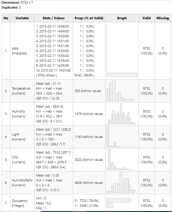
Observations
All environmental variables are read correctly as numeric type by R, however, we need to define a variable “date” as of date class type. For the ‘Date’ variable treatment, we use the “lubridate” package. Also, we have daytime information available in the date column which we can extract and use for modeling as occupancy for spaces like offices will depend on daytime. Another important observation is that we don’t have missing values in the entire dataset. An Occupancy variable needs to be defined as a factor type for further analysis.
library("readr")
library("lubridate")
data$date1 = as_date(data$date)
data$date= as.POSIXct(data$date, format = "%Y-%m-%d %H:%M:%S")
data$time = format(data$date, format = "%H:%M:%S")
data1= data[,-1]
data1$Occupancy = as.factor(data1$Occupancy)
Now our processed data looks like this:
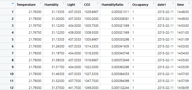
Processed Data Preview
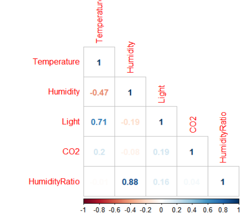
Next, we check two important aspects of data, one is the correlation plot of variables to understand multicollinearity issues in the dataset and the proportion of target variable distribution.
library(corrplot)
numeric.list <- sapply(data1, is.numeric)
numeric.list
sum(numeric.list)
numeric.df <- data1[, numeric.list]
cor.mat <- cor(numeric.df)
corrplot(cor.mat, type = "lower", method = "number")
library(plotrix)
pie3D(prop.table((table(data1$Occupancy))), main = "Occupied Vs Unoccupied", labels=c("Unoccupied","Occupied"), col = c("Blue", "Dark Blue"))
Pie Chart for Occupancy
From the correlation plot, we observe that temperature and light are positively correlated while temperature and Humidity are negatively correlated, humidity and humidity ratio are highly correlated which is obvious as the Humidity ratio is the ratio of Humidity and temperature. Hence while building various models we will consider variable Humidity and omit Humidity ratio.
Now we are all set for model building. As our response variable Occupancy is binary, we need classification types of models. Here we implement CART, RF, and ANN.
Model Building- Classification and Regression Trees (CART): Now we define training and test datasets in the required format for model building.
p_train = data1
p_test = read.csv("datatest2.txt",header = T, sep = ",", row.names = 1)
p_test$date1 = as_date(p_test$date)
p_test$date= as.POSIXct(p_test$date, format = "%Y-%m-%d %H:%M:%S")
p_test$time = format(p_test$date, format = "%H:%M:%S")
p_test= p_test[,-1]
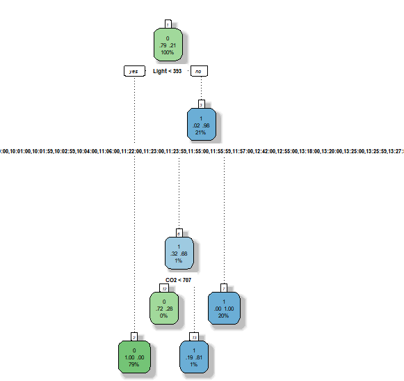
Note that the R implementation of the CART algorithm is called RPART (Recursive Partitioning And Regression Trees) available in a package of the same name. The algorithm of decision tree models works by repeatedly partitioning/splitting the data into multiple sub-spaces so that the outcomes in each final sub-space are as homogeneous as possible.
The model uses different splitting rules that can be used to effectively predict the type of outcome. These rules are produced by repeatedly splitting the predictor variables, starting with the variable that has the highest association with the response variable. The process continues until some predetermined stopping criteria are met. We define these stopping criteria using control parameters such as a minimum number of observations in a node of the tree before attempting a split, a split must decrease the overall lack of fit by a factor before being attempted.
library(rpart)
library(rpart.plot)
library(rattle)
#Setting the control parameters
r.ctrl = rpart.control(minsplit=100, minbucket = 10, cp = 0, xval = 10)
#Building the CART model
set.seed(123)
m1 <- rpart(formula = Occupancy~ Temperature+Humidity+Light+CO2+date1+time, data = p_train, method = "class", control = r.ctrl)
#Displaying the decision tree
fancyRpartPlot(m1).
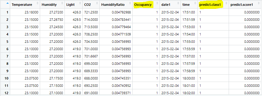
Now we predict the occupancy variable for the test dataset using predict function.
p_test$predict.class1 <- predict(ptree, p_test[,-6], type="class")
p_test$predict.score1 <- predict(ptree, p_test[,-6], type="prob")
View(p_test)
Now evaluate the performance of our model by plotting the ROC curve and building a confusion matrix.
library(ROCR)
pred <- prediction(p_test$predict.score1[,2], p_test$Occupancy)
perf <- performance(pred, "tpr", "fpr")
plot(perf,main = "ROC curve")
auc1=as.numeric(performance(pred, "auc")@y.values)
library(caret)
m1=confusionMatrix(table(p_test$predict.class1,p_test$Occupancy), positive="1",mode="everything")
Here we get an AUC of 82% and a model accuracy of 98.1%.
Now next in the list is Random Forest. In the random forest approach, a large number of decision trees are created. Every observation is fed into every decision tree. The most common outcome for each observation is used as the final output. A new observation is fed into all the trees and taking a majority vote for each classification model. The R package “randomForest” is used to create random forests.
RFmodel = randomForest(Occupancy~Temperature+Humidity+Light+CO2+date1+time, data = p_train1, mtry = 5, nodesize = 10, ntree = 501, importance = TRUE)
print(RFmodel)
plot(RFmodel)
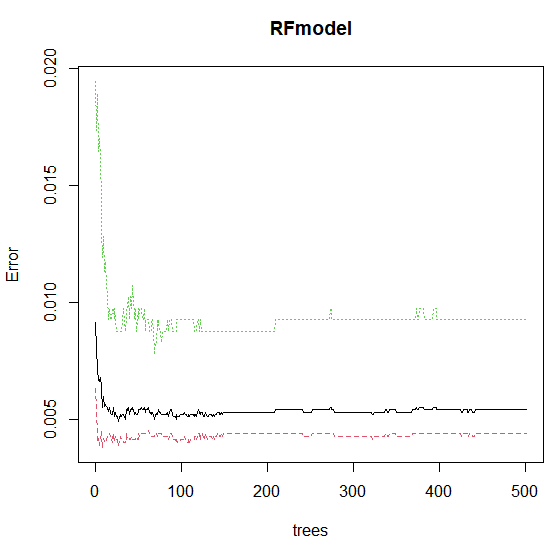
Here we observe that error remains constant after n=150, so we can tune the model with trees 150.
Also, we can have a look at important variables in the model which are contributing to occupancy detection.
importance(RFmodel)
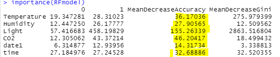
We observe from the above output that light is the most important predictor followed by CO2, Temperature, Time, Humidity, and date when we consider accuracy. Now, let’s prune the RF model with new control parameters.
set.seed(123)
tRF=tuneRF(x=p_train1[,-c(5,6)],y=as.factor(p_train1$Occupancy), mtryStart = 5, ntreeTry = 150, stepFactor = 1.15, improve = 0.0001, trace = TRUE, plot = TRUE, doBest = TRUE, nodesize=10, importance= TRUE)
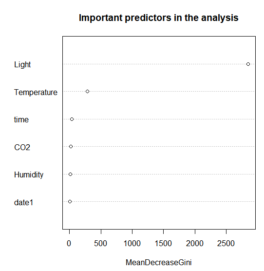
Now with this tuned model we again variable importance as follows. Please note here variable importance is measured for decreasing Gini Index, however earlier it was a mean decrease in model accuracy.
varImpPlot(tRF,type=2, main = "Important predictors in the analysis")
Now next we predict occupancy for the test dataset using predict function and tuned RF model.
p_test1$predict.class= predict(tRF, p_test1, type= "class")
p_test1$predict.score= predict(tRF, p_test1, type= "prob")
We check the performance of this model using the ROC curve and confusion matrix parameters. The AUC turns out to be 99.13% with a very stiff curve as below and the accuracy of prediction is 98.12%.
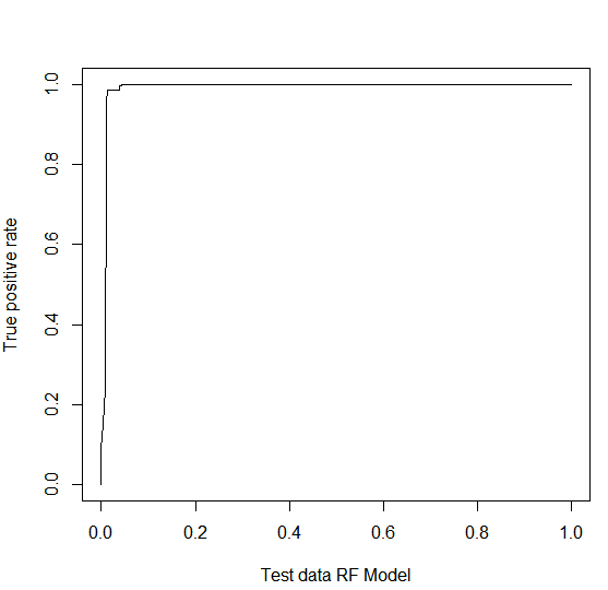
It seems like this model is doing better than the CART model. Time to check ANN!
Now we build an artificial neural network for the classification. Neural Network (or Artificial Neural Network) has the ability to learn by examples. ANN is an information processing model inspired by the biological neuron system. It is composed of a large number of highly interconnected processing elements known as the neuron to solve problems.
Here I am using the ‘neuralnet’ package in R. When we try to build ANN for our case, we observe that the model does not accept date class variables we will omit them. Another way could be we create a separate factor variable from the daytime variable with levels like Morning, Afternoon, Evening, and Night and then create a dummy variable for the factor variable.
Before actually building ANN, we need to scale our data as variables have values in different ranges. ANN being a weight-based algorithm, maybe biased results if data is not scaled.
p_train2=p_train2[,-c(6,7,8)]
p_train_sc=scale(p_train2)
p_train_sc = as.data.frame(p_train_sc)
p_train_sc$Occupancy=data1$Occupancy
p_test3=p_test2[,-c(6,7,8)]
p_test_sc=scale(p_test3)
p_test_sc = as.data.frame(p_test_sc)
p_test_sc$Occupancy=p_test2$Occupancy
After scaling all the variables (except Occupancy) our data will look like this.
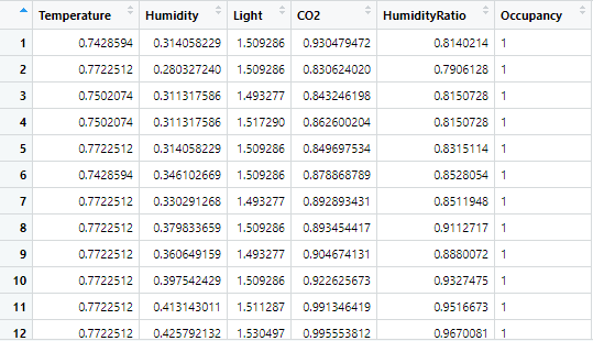
Now we are all set for model building.
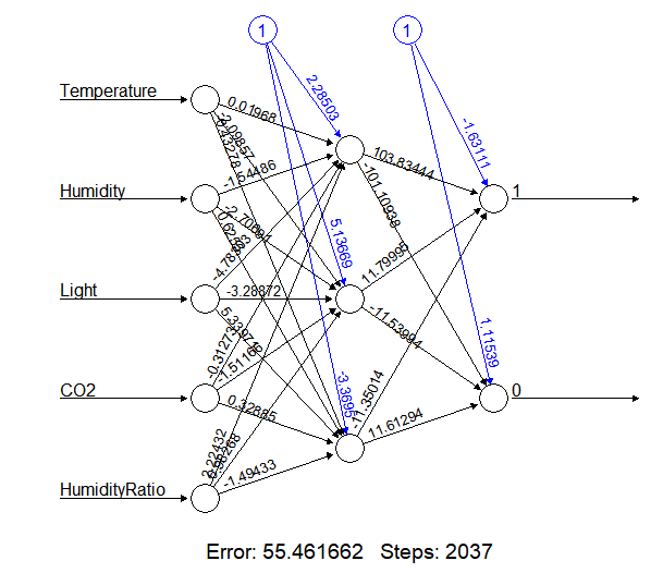
nn1 = neuralnet(formula = Occupancy~Temperature+Humidity+Light+CO2+HumidityRatio, data = p_train_sc,
                hidden = 3, err.fct = "sse",linear.output = FALSE,lifesign = "full",
                lifesign.step = 10, threshold = 0.03, stepmax = 10000)
plot(nn1)
We calculate results for the test dataset using Compute function.
compute.output = compute(nn1, p_test_sc[,-6])
p_test_sc$Predict.score <- compute.output$net.result
p_test_sc$Class = ifelse(p_test_sc$Predict.score[,1]>0.5,0,1)
Models Performance Comparison: We again evaluate this model using the confusion matrix and ROC curve. I have tabulated results obtained from all three models as follows:
| Performance measure | CART on a test dataset | RF on a test dataset | ANN on a test dataset |
| AUC | 0.8253 | 0.9913057 | 0.996836 |
| Accuracy | 0.981 | 0.9812 | 0.9942 |
| Kappa | 0.9429 | 0.9437 | 0.9825 |
| Sensitivity | 0.9514 | 0.9526 | 0.9951 |
| Specificity | 0.9889 | 0.9889 | 0.9939 |
| Precision | 0.9586 | 0.9587 | 0.9775 |
| Recall | 0.9514 | 0.9526 | 0.9951 |
| F1 | 0.9550 | 0.9556 | 0.9862 |
| Balanced Accuracy | 0.9702 | 0.9708 | 0.9945 |
From performance measures comparison, we observe that ANN outperforms other models, followed by RF and CART. With machine earning algorithms we can replace occupancy sensor functionality efficiently with good accuracy.
The media shown in this article are not owned by Analytics Vidhya and are used at the Author’s discretion.


