This article was published as a part of the Data Science Blogathon
Introduction
The ultimate goal of this blog is to predict the sentiment of a given text using python where we use NLTK aka Natural Language Processing Toolkit, a package in python made especially for text-based analysis. So with a few lines of code, we can easily predict whether a sentence or a review(used in the blog) is a positive or a negative review.

Before moving on to the implementation directly let me brief the steps involved to get an idea of the analysis approach. These are namely:
1. Importing Necessary Modules
2. Importing Dataset
3. Data Preprocessing and Visualization
4. Model Building
5. Prediction
So let’s move on focussing each step in detail.
1. Importing Necessary Modules:
So as we all know that it is necessary to import all the modules which we are going to use initially. So let’s do that as the first step of our hands-on.
Here we are importing all the basic import modules required namely numpy, pandas, matplotlib, seaborn and beautiful soup each having its own use case. Though we are going to use a few other modules excluding these let’s understand them while we use them.
2. Importing Dataset:
I had actually downloaded the dataset from Kaggle quite a long time back hence I don’t have the link to the dataset. So to get the dataset as well as the code I will put the Github repo link so that everyone has access to it. Now to import the dataset we have to use the pandas method ‘read_csv’ followed by the file path.
If print the dataset we could see that there are ‘568454 rows × 10 columns’ which is quite big.
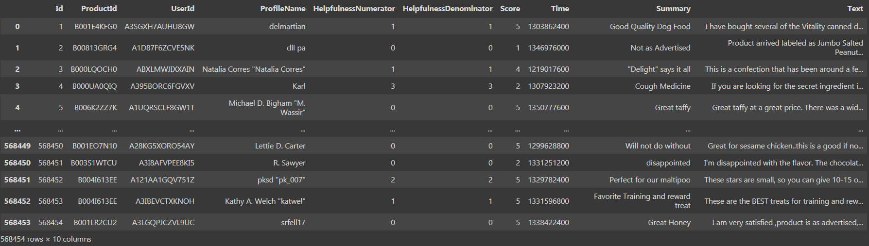
We see that there are 10 columns namely ‘Id’, ‘HelpfulnessNumerator’, ‘HelpfulnessDenominator’, ‘Score’ and ‘Time’ as datatype int64 and ‘ProductId’, ‘UserId’, ‘ProfileName’, ‘Summary’, ‘Text’ as object datatype. Now let’s move on to the third step i.e. Data Preprocessing and Visualisation.
import numpy as np                  #linear algebra
import pandas as pd                 # data processing, CSV file I/O (e.g. pd.read_csv)
import matplotlib.pyplot as plt     #For Visualisation
import seaborn as sns               #For better Visualisation
from bs4 import BeautifulSoup       #For Text Parsing
data = pd.read_csv('Reviews.csv')
print(data.shape)
3. Data Preprocessing and Visualisation:
Now we have access to the data after which we have clean the data. Using the ‘isnull().sum()’ method we could easily find the total number of missing values in the dataset.
data.isnull().sum()
If we execute the above code as a cell we find that there are 16 and 27 null values in the ‘ProfileName’ and ‘Summary’ columns respectively. Now, we have to either replace the null values with the central tendency or remove the respective rows which contain the null values. With such a vast number of rows removing just 43 rows that contain the null values wouldn’t affect the overall accuracy of the model. Hence it is wise to remove the 43 rows using the ‘dropna’ method.
data = data.dropna()
Now, I have updated the old data frame rather than creating a new variable and storing the new data frame with the cleaned values. Now again when we check the data frame we find that there are 568411 rows and the same 10 columns, meaning the 43 rows which had the null values have been dropped and now our dataset is cleaned. Proceeding further we have to do some preprocessing of the data in such a way that it could be directly used by the model.
To preprocess we use the ‘Score’ column in the data frame to have scores ranging from ‘1’ to ‘5’, where ‘1’ means a negative review and ‘5’ means a positive review. But it is better to have the score initially ranging from ‘0 ‘to ‘2 ‘where ‘0’ means a negative review, ‘1’ means a neutral review and ‘2’ means a positive review. It is similar to encoding in python but here we don’t use any in-built function but we explicitly run a for loop where and create a new list and append the values to the list.
a=[]
for i in data['Score']:
    if i <3:
        a.append(0)
    if i==3:
        a.append(1)
    if i>3:
        a.append(2)
Supposing the ‘Score’ lies in the range of ‘0’ to ‘2’ we consider those as negative reviews and append them to the list with a score of ‘0’ meaning negative review. Now if we plot the values of the scores present in the list ‘a’ as the nomenclature used above we find that there are 82007 negative reviews, 42638 neutral reviews, and 443766 positive reviews. We can clearly find that approximately 85% of the reviews in the dataset have positive reviews and the remaining are either negative or neutral reviews. This could be visualized and understood more clearly with the help of a countplot in the seaborn library.
sns.countplot(a)
plt.xlabel('Reviews', color = 'red')
plt.ylabel('Count', color = 'red')
plt.xticks([0,1,2],['Negative','Neutral','Positive'])
plt.title('COUNT PLOT', color = 'r')
plt.show()
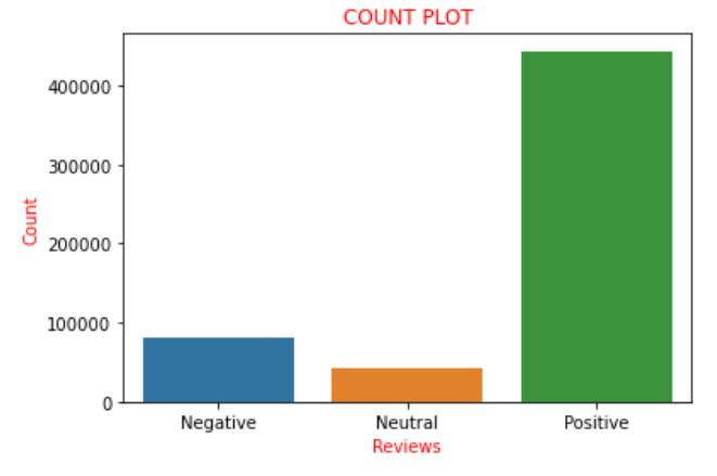
Therefore the above plot clearly portrays all the sentences described earlier pictorially. Now I convert the list ‘a’ which we had encoded earlier into a new column named ‘sentiment’ to the data frame i.e. ‘data’. Now there comes a twist where we create a new variable say ‘final_dataset’ where I consider only the ‘Sentiment’ and ‘text’ column of the data frame which is the new data frame that we are going to work on for the forthcoming part. The reason behind it is that all the remaining columns are regarded as those that don’t contribute to the sentiment analysis hence without dropping them we consider the data frame excluding those columns. Hence, that is the reason for choosing only the ‘Text’ and the ‘Sentiment’ columns. We code the same thing as below:
data['sentiment']=a
final_dataset = data[['Text','sentiment']]
final_dataset
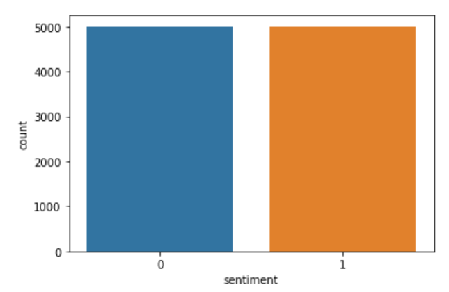
Now if we print the ‘final_dataset’ and find the shape we come to know that there are 568411 rows and only 2 columns. From the final_dataset if we find out the number of positive reviews is 443766 entries and the number of negative reviews is found to be 82007. Hence there is a very large difference between the positive and negative reviews. Hence, there are more chances for the data to overfit if we directly try to build the model. Therefore, we have to choose only a few entries from the final_datset to avoid overfitting. So from various trials, I have found that the optimal value for the number of reviews to be considered is 5000. Hence I create two new variables ‘datap’ and ‘datan’ and store randomly any 5000 positive and negative reviews in the variables respectively. The code implementing the same is below:
datap = data_p.iloc[np.random.randint(1,443766,5000), :]
datan = data_n.iloc[np.random.randint(1, 82007,5000), :]
len(datan), len(datap)
Now I create a new variable named data and concatenate the values in ‘datap’ and ‘datan’.
data = pd.concat([datap,datan])
len(data)
Now I create a new list named ‘c’ and what I do is similar to encoding but explicitly. I store the negative reviews ‘0’ as ‘0’ and positive reviews ‘2’ earlier as ‘1’ in ‘c’. Then again I replace the values of the sentiment stored in ‘c’ in the column data. Then to view whether the code has run properly I plot the ‘sentiment’ column. The code implementing the same thing is:
c=[]
for i in data['sentiment']:
    if i==0:
        c.append(0)
    if i==2:
        c.append(1)
data['sentiment']=c
sns.countplot(data['sentiment'])
plt.show()
If we see the data then we can find that there are a few HTML tags since the data was originally fetched from real e-commerce sites. Hence we can find that there are tags present which is to be removed as they are not necessary for the sentiment analysis. Hence we use the BeautifulSoup function which uses the ‘html.parser’ and we can easily remove the unwanted tags from the reviews. To perform the task I create a new column named ‘review’ which stores the parsed text and I drop the column named ‘sentiment’ to avoid redundancy. I have performed the above task using a function named ‘strip_html’. The code to perform the same is as follows:
def strip_html(text):
    soup = BeautifulSoup(text, "html.parser")
    return soup.get_text()
data['review'] = data['Text'].apply(strip_html)
data=data.drop('Text',axis=1)
data.head()
Now we have come to the end of a tiresome process of Data Preprocessing and Visualization. Hence we can now proceed with the next step i.e. Model Building.
4. Model Building:
Before directly we jump to building the model we need, to just do a small task. We know that for humans to classify the sentiment we need articles, determinants, conjunctions, punctuation marks, etc, as we can clearly understand and then classify the review. But this is not the case with machines So they don’t actually need these to classify the sentiment rather they just get confused literally if they are present. So to perform this task like any other sentiment analysis we need to use the ‘nltk’ library. NLTK stands for ‘Natural Language Processing Toolkit’. This is one of the core libraries to perform Sentiment Analysis or any text-based ML Projects. So with the help of this library, I am going first remove the punctuation marks and then remove the words which do not add a sentiment to the text. First I use a function named ‘punc_clean’ which removes the punctuation marks from every review. The code to implement the same is below:
import nltk
def punc_clean(text):
    import string as st
    a=[w for w in text if w not in st.punctuation]
    return ''.join(a)
data['review'] = data['review'].apply(punc_clean)
data.head(2)
Therefore the above code removes the punctuation marks. Now next we have to remove the words which don’t add a sentiment to the sentence. Such words are called the ‘stopwords’. The list of almost all the stopwords could be found here. Next, if we go through the list of the stopwords we can find that it contains the word ‘not’ as well. So it is necessary that we don’t remove the ‘not’ from the ‘review’ as it adds some value to the sentiment because it contributes to the negative sentiment. Hence we have to write the code in such a way that we remove other words except the ‘not’. The code to implement the same is:
def remove_stopword(text):
    stopword=nltk.corpus.stopwords.words('english')
    stopword.remove('not')
    a=[w for w in nltk.word_tokenize(text) if w not in stopword]
    return ' '.join(a)
data['review'] = data['review'].apply(remove_stopword)
Therefore we have now just a step behind the model building. The next motive is to assign each word in every review with a sentiment score. So to implement it we need to use another library from the ‘sklearn’ module which is the ‘TfidVectorizer’ which is present inside the ‘feature_extraction.text’. It is highly recommended to go through the ‘TfidVectorizer’ docs to get a clear understanding of the library. It has many parameters like input, encoding, min_df, max_df, ngram_range, binary, dtype, use_idf, and much more parameters each having its own use case. Hence it is recommended to go through this blog to get a clear understanding of the working of ‘TfidVectorizer’. The code which implements the same is:
from sklearn.feature_extraction.text import TfidfVectorizer
vectr = TfidfVectorizer(ngram_range=(1,2),min_df=1)
vectr.fit(data['review'])
vect_X = vectr.transform(data['review'])
Now it’s time to build the model. Since it is a binary class classification sentiment analysis i.e. ‘1’ referring to a positive review and ‘0’ referring to a negative review. So it is clear that we need to use any of the Classification Algorithm. The one used here is the Logistic Regression. Hence we need to import ‘LogisticRegression’ to use it as our model. Then we need to fit the entire data as such because I felt that it is nice to test the data from entirely new data rather than from the available dataset. So I have fitted the entire dataset. Then I use the ‘.score()’ function to predict the score of the model. The code implementing the above-mentioned tasks is as given below:
from sklearn.linear_model import LogisticRegression
model = LogisticRegression()
clf=model.fit(vect_X,data['sentiment'])
clf.score(vect_X,data['sentiment'])*100
If we run the above piece of code and check the score of the model we get around 96 – 97% as the dataset changes every time we run the code as we consider the data randomly. Hence we have successfully built our model that too with a good score. Then why wait to test how our model performs in the real-world scenario. So now we move on to the last and final step of the ‘Prediction’ to test our model’s performance.
5. Prediction:
So to clarify the performance of the model I have used two simple sentences “I love icecream” and “I hate icecream” which clearly refer to positive and negative sentiment. The output is as follows:
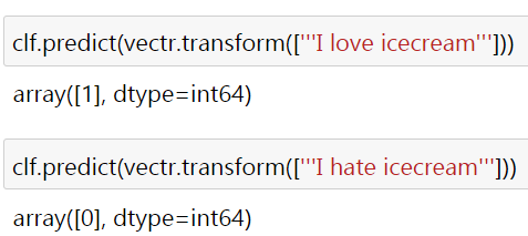
Here the ‘1’ and ‘0’ refer to the positive and the negative sentiment respectively. Why not a few real-world reviews be tested. I request you as readers to check and test out the same. You would mostly get the desired output but if that doesn’t work I request you to try changing the parameters of the ‘TfidVectorizer’ and do model tuning to ‘LogisticRegression’ to get the required output. So for which I have attached the link to the code and the dataset here.
You connect with me through linkedin. Hope this blog is useful to understand how a Sentiment Analysis is done practically with the help of Python codes as well. Thanks for viewing the blog.
A seasoned software and ML developer with likes to share knowledge on the latest skills, frameworks, and technologies. Writes about Data Science and Machine learning and love to build and ship projects.


